We See Risk Where Others May Not: Applying Dynamic Risk Management to a Cash Equities Portfolio

1. Introduction

Risk management can, we strongly believe, successfully guide investment decision making. Principally: (i) diversification should play a central role in constructing a portfolio; and (ii) systematic risk management can be used to improve a portfolio’s risk-adjusted returns and tail characteristics. Crucially, we believe that it is possible to forecast risks much more accurately than returns. Diversification can be achieved by balancing risks within the portfolio, and there is additional benefit to be gained from systematically mitigating overall portfolio risk. In this article, we translate this philosophy over to a new investment problem: managing a portfolio of global stocks. We investigate risk-based techniques to build stock portfolios from the bottom up, and then to systematically manage overall portfolio risk from the top down. Our aim is to improve expected returns for lower downside risk compared to a conventional capitalisation-weighted (cap-weighted) index.

Our approach can be broken down into four steps, which are summarised in terms of risk and return in Figure 1:

1. Market: Begin with a conventional cap-weighted index, such as the MSCI World Index;
2. Risk Aware: Use portfolio-optimisation techniques to improve the portfolio’s diversification and risk characteristics. The resulting portfolio aims to deliver comparable returns to the MSCI World Index, for considerably lower volatility;
3. Risk Aware Levered: Use leverage to increase expected returns of the Risk Aware portfolio and bring its beta close to that of the MSCI World Index. The resulting portfolio has similar risk characteristics to the MSCI World Index, but higher expected returns;
4. Risk Managed: Use risk overlays to systematically manage overall portfolio risk. Each risk overlay addresses a specific risk faced by the portfolio, improving tail characteristics.

Figure 1. Applying Risk-Management Theory to Equities

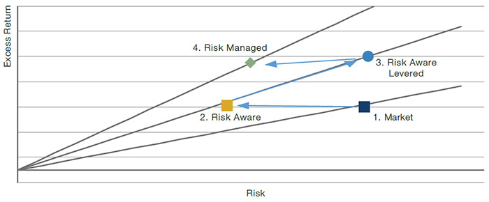
Source: Man Group. For illustrative purposes.

2. Optimal Portfolios Without Return Forecasts

By construction, cap-weighted indices tend to concentrate in the largest stocks (Figure 2). Importantly, the weight for each stock is determined without reference to its risk or to the diversification benefit it may offer a portfolio. Individual stock risk and diversification benefit clearly play important roles in the overall risk of a portfolio. We believe that an investor can reliably incorporate this information into portfolio construction to improve risk-adjusted returns.

Figure 2. Index Concentration by Decile

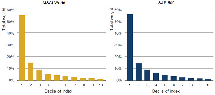
Source: Man Group, Bloomberg; as of September 2020.

Rational finance teaches us that investors bearing higher (undiversifiable) risk should be rewarded with higher expected returns. In multi-asset investing, there is empirical evidence to support this. For example, in the US, equity returns have been higher and more volatile than bond returns, which, in turn, have been higher and more volatile than cash returns.¹ There are various approaches to risk parity investing, but they are typically based on the assumption that asset classes have similar Sharpe ratios going forward. Or, in other words, the expected excess return of an asset class is proportional to its volatility.

This assumption of the proportionality of risk and return is harder to justify in single stock investing. Historically, high risk stocks have, on average, performed only slightly better than low volatility stocks. This is true whether risk is interpreted as either volatility or market beta and invalidates the classical capital asset pricing model (‘CAPM’). This observation, illustrated in Figure 3, is sometimes described as the ‘security market line’ being flatter than what the CAPM implies, and has long been documented.² Academic explanations for this phenomenon include the existence of leverage restrictions³ and the prevalence of benchmarking among institutional investors.

Figure 3. Risk-Return Relationship for Stocks

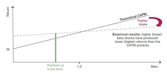
Source: Man Group. For illustrative purposes only. This figure illustrates how the empirical results compare to the CAPM in beta-return space. In this diagram, Rf is the risk-free rate.

Given the uncertainty around the risk-return relationship of stocks, we base our approach on the more tractable characteristics of correlation and volatility in building a risk-based (‘Risk Aware’) portfolio, without the need for return forecasts. We believe this approach builds a portfolio that harvests the equity risk premium with lower risk (i.e. with a higher Sharpe ratio) than passive approaches, while not relying on return forecasts for individual stocks.

2.1. Risk Estimation

Although we do not need to estimate expected returns for the Risk Aware portfolio, we do need to estimate the covariance of stock returns. There are some well-known difficulties associated with estimating covariance matrices for portfolio optimisations. First, optimisation solutions can be very sensitive to small changes in the covariance matrix. This can also be described as a lack of statistical robustness. Second is the curse of dimensionality. For a universe of n assets, a covariance matrix effectively represents a set of n(n+1)/2 parameters. A large number of parameters requires a large amount of data to estimate reliably, and, in this case, the number of parameters grows faster than the number of assets. This poses a problem for portfolios of stocks, where the investment universe may number thousands of assets.

We employ two methods to reduce the dimensionality of covariance estimation and improve statistical robustness. The first method uses a factor model. We use principal component analysis to identify the most important statistical factors driving stock returns. We then estimate covariances from stock volatilities and factor exposures. In the second method, we use hierarchical clustering to regularise a traditionally computed covariance matrix. The clustering identifies nested groups of stocks based on their co-movement. We smooth the correlations between groups by averaging. The smoothing effectively reduces the number of model parameters, improving robustness. Figure 4 provides an example of a covariance matrix smoothed via hierarchical clustering.

Figure 4. Hierarchical Clustering

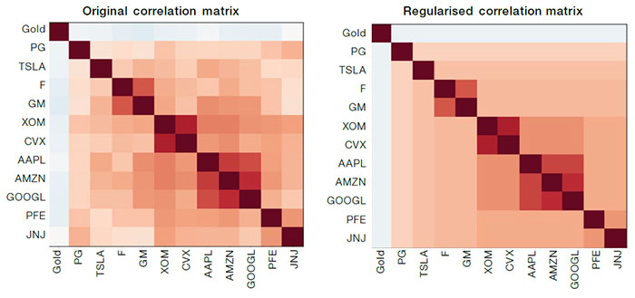
Source: Man Group, Bloomberg; as of September 2020.
The algorithm creates clusters of highly correlated stocks. For example, Apple (‘AAPL’), Amazon (‘AMZN’) and Alphabet (‘GOOGL’) are grouped in the same cluster.

2.2. Risk Aware: The Long-Term Evidence

As a justification for the blended approach, we present long-term evidence on the performance of the hypothetical Risk Aware approach over a cap-weighted benchmark. We use the Center for Research in Security Prices (‘CRSP’) dataset of US stocks between 1968 and 2014 to create the hypothetical Risk Aware portfolio.⁴ We then test the factor-based and hierarchical clustering approaches separately, imposing a maximum weight constraint of 100 basis points.

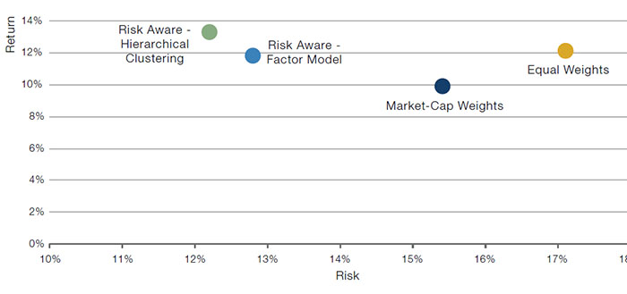
Table 1 shows that the Risk Aware portfolio exhibits, for both methods, improved maximum drawdowns and higher risk-adjusted returns (information ratio) relative to a cap-weighted or equal-weighted portfolio. This point is also illustrated in Figure 5 and Figure 6, where higher returns are achieved for lower risk than the cap-weighted portfolio or the equal-weighted portfolio, whether we use a factor model or hierarchical clustering.

Table 1. Long-Term Backtest – Factor Model

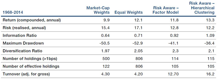
Source: Man Group, CRSP; between 1968 and 2014.

Figure 5. Long-Term Backtest – Factor Model and Hierarchical Clustering

Simulated past performance is not indicative of future results. Returns may increase or decrease as a result of currency fluctuations.
Source: Man Group, CRSP; between 1968 and 2014.
Simulated performance data and hypothetical results are shown for illustrative purposes only, do not reflect actual trading results, have inherent limitations and should not be relied upon. Results are gross of any fees or expenses which could materially reduce returns. Please see the end of this paper for additional important information on simulated results.

2.3. Adding an ESG Tilt to the Portfolios

It is straightforward to include ESG constraints as part of the Risk Aware portfolio construction. We impose the following:

• Minimum ESG score: We use Man Numeric’s methodology to calculate an ESG score for each company. The methodology generates scores which are neutral on a country, sector and industry level. The scores are then aggregated at a portfolio level. We constrain the portfolio to have a minimum portfolio-level score;
• Low-carbon constituents: We use data from TruCost for the carbon intensity of each company. This is a measure of the CO2 emissions the company generates as part of its activities. We set a maximum level of emissions that companies must not exceed to be considered for inclusion in the portfolio. This constraint can have a material impact on certain sector or industry exposures (for example, utility companies will tend to be underweighted). However, in the case of the Risk Aware strategy, the performance impact is minimal.

2.4. Simulation Results

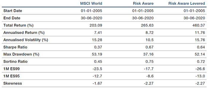
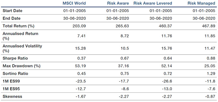
Referring back to Figure 1, the Risk Aware portfolio, shifts us up slightly (higher return) and to the left (lower risk) of the market portfolio. Table 2 shows some performance and risk statistics for the hypothetical Risk Aware portfolio, based on a universe of global stocks for the period from January 2005 to June 2020.⁵ Figure 6 compares the performance of the hypothetical Risk Aware portfolio to the market.

Table 2. Backtest Results

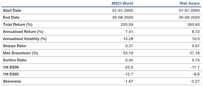
Source: Man Group, Bloomberg; between January 2005 and June 2020.
All metrics use end-of-month monthly returns except for 1M ES95, 1M ES99, and Skewness (using 20-day overlapping returns).

Figure 6. Compounded Returns (Log Scale)

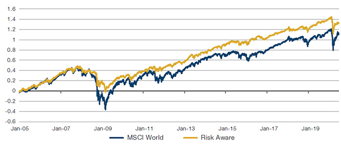
Simulated past performance is not indicative of future results. Returns may increase or decrease as a result of currency fluctuations.
Source: Man Group, Bloomberg; between January 2005 and June 2020.
Simulated performance data and hypothetical results are shown for illustrative purposes only, do not reflect actual trading results, have inherent limitations and should not be relied upon. Results are gross of any fees or expenses which could materially reduce returns. Please see the end of this paper for additional important information on simulated results.

3. Leverage: Benefits, Costs and Risks

The Risk Aware portfolio seeks to improve upon the risk properties of a cap-weighted portfolio, without compromising expected returns. It has a lower volatility than the MSCI World Index, but leverage can be applied to adjust for this. In this case, we define risk as the Barra Global Beta of the portfolio, as shown in Figure 7. We also show the Barra Global Beta of a version of the Risk Aware portfolio that has been levered up by a factor of 1.5, bringing its risk closer to that of the MSCI World Index. As shown in Figure 1, the use of leverage moves the portfolio towards the top right corner in risk-return space; expected returns increase in proportion with portfolio risk.

Figure 7. Barra Global Betas

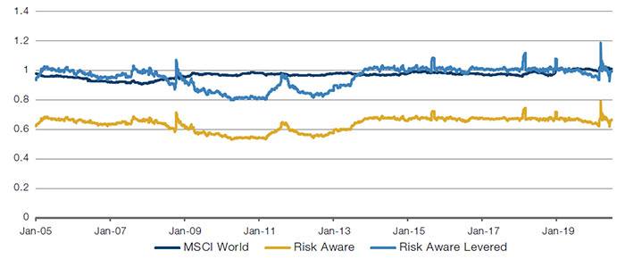
Source: Man Group, Bloomberg, Barra; between January 2005 and June 2020.

Table 3 compares some performance and risk statistics of the levered portfolio with the MSCI World Index, and Figure 8 charts the performance.

Table 3. Backtest Results

Source: Man Group, Bloomberg; between January 2005 and June 2020.
All metrics use end-of-month monthly returns except for 1M ES95, 1M ES99, and Skewness (using 20-day overlapping returns).

Figure 8. Cumulative Returns (Log Scale)

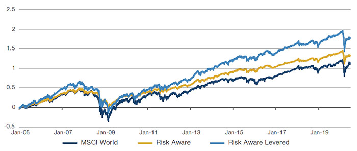
Simulated past performance is not indicative of future results. Returns may increase or decrease as a result of currency fluctuations.
Source: Man Group, Bloomberg; between January 2005 and June 2020.
Simulated performance data and hypothetical results are shown for illustrative purposes only, do not reflect actual trading results, have inherent limitations and should not be relied upon. Results are gross of any fees or expenses which could materially reduce returns. Please see the end of this paper for additional important information on simulated results.

Leverage has the benefit of magnifying the returns of the portfolio. However, it also has some costs. First, there is a financing cost, which is typically greater than the return on cash.⁶ Second, there is a cost associated with increased tail loss: Figure 9 shows that, during the worst 1-day returns experienced by the MSCI World, the Risk Aware Levered portfolio tended to experience equally bad or worse returns. This is because the returns of the Risk-Aware portfolio are more negatively skewed than those of the MSCI World, as we can observe in Table 3.⁷ The good news is, however, that tail losses, like any other kind of risk, can be managed with the right toolkit. This is the subject of the next section.

Figure 9. Returns During Worst 1-Day MSCI World Selloffs

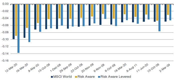
Simulated past performance is not indicative of future results. Returns may increase or decrease as a result of currency fluctuations.
Source: Man Group, Bloomberg; between January 2005 and June 2020.
Simulated performance data and hypothetical results are shown for illustrative purposes only, do not reflect actual trading results, have inherent limitations and should not be relied upon. Results are gross of any fees or expenses which could materially reduce returns. Please see the end of this paper for additional important information on simulated results.

4. Dynamic Exposure Control: Risk Overlays for a Long-Only Equity Portfolio

We now introduce a set of systematic overlays to address some risks faced by long-only stocks portfolios. We apply these overlays to the Risk Aware Levered portfolio. The objective here is to control market beta in a responsive yet cost-efficient manner. To this end, systematic overlays are implemented with equity index futures, taking short positions to offset aggregate risk from the stocks portfolio. The equity index futures are weighted to match the regional exposures of the Risk Aware Levered portfolio, shown in Table 4.

Table 4. Index Futures Allocations

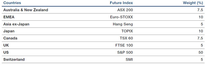
Source: Man Group, Bloomberg; between January 2005 and June 2020

4.1. Risk Overlays

The objective of the risk overlays is to reduce portfolio risk in periods of heightened market stress, and thus improve risk-adjusted returns and tail properties. Reducing risk effectively means reducing exposure, and so reducing the potential to earn the equity risk premium. For the risk overlays to be effective, they must reduce portfolio risk more than they reduce portfolio returns. Referring to Figure 1, we are looking to move southwest in risk-return space, but at a shallower gradient than simply reducing leverage. That is, we want to move farther left (lower risk) than we move down (lower return). The four risk overlays we consider are:

• Volatility-switching overlay: We estimate two volatilities for the Risk Aware Levered portfolio – a fast one and a slow one. The fast measure rising significantly above the slow measure indicates a volatility spike, and an increased risk of an equity selloff. The volatility switching overlay reduces portfolio risk in these scenarios: the larger the spike, the larger the risk reduction;
• Momentum overlay: Trend signals are monitored for each of the equity index futures traded. Moderate-to-strong down trends are associated with additional regional downside risk. In these scenarios, risk in the corresponding regions is reduced by shorting the relevant futures contract;
• Correlation overlay: We utilise a high-frequency correlation model to help spot when a bond sell-off can potentially spill over into equities;
• Diversification-benefit overlay: Using high-frequency stock data, we measure market breadth through stock correlations. An increase in stock correlations represents a reduction in market breadth or, equivalently, a loss of diversification potential. In these scenarios, there is a heightened risk of an equity selloff, and the diversification-benefit overlay reduces portfolio risk.

Figure 10 illustrates the behaviour of the four risk overlays by showing the amount by which each wants to cut the exposure of the Risk Aware Levered portfolio. Figure 11 shows the resulting net exposure of a portfolio combining the Risk Aware Levered portfolio with the systematic overlays. The combination is achieved by adding 1 to each of the degear factors, calculating their product, and subtracting 1 from the result. This number is then further adjusted to respect exposure constraints, a process explained more in depth in the next subsection.

Figure 10. Degear Amounts (as % of Risk Aware Levered Portfolio)

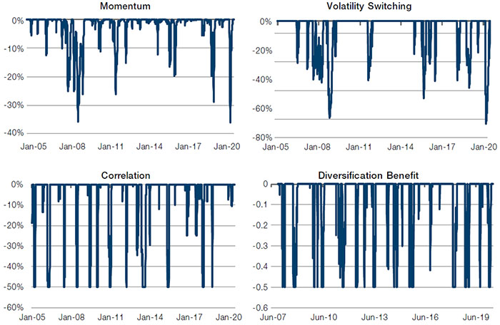
Source: Man Group; between January 2005 and June 2020.

Figure 11. Net Exposure (%) of the Risk Aware Levered portfolio Plus the Risk Overlays

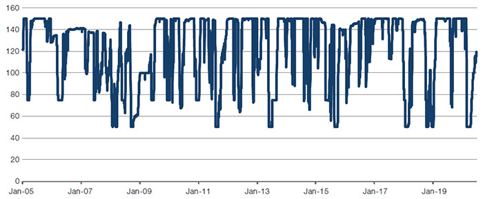
Source: Man Group; between January 2005 and June 2020.

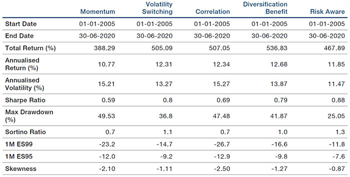
Table 5 gives some performance and risk statistics for the Risk Aware Levered portfolio on its own, with each of the risk overlays, and with all the risk overlays combined. Two observations are in order:

• Applying risk overlays tends to reduce portfolio volatility. This is to be expected, as the application of risk overlays results in lower average exposures;
• Overlays should not be expected to increase returns. Even though our simulation showed an improvement in returns, this will not necessarily continue in the future. This is acceptable since we are willing to forego returns if we can obtain an improvement in risk-adjusted performance (such as an improvement in Sharpe ratio or better tail properties as measured by skewness, expected shortfall or maximum drawdown). Additional returns come through managed leverage.

Table 5. Adding Risk Overlays to the Risk Aware Levered Portfolio (One at a Time and in Combination) – Backtest Results

Simulated past performance is not indicative of future results. Returns may increase or decrease as a result of currency fluctuations.
Source: Man Group, Bloomberg; between January 2005 and June 2020.
Simulated performance data and hypothetical results are shown for illustrative purposes only, do not reflect actual trading results, have inherent limitations and should not be relied upon. Results are gross of any fees or expenses which could materially reduce returns. Please see the end of this paper for additional important information on simulated results.

4.2. Exposure Constraints

After the risk overlays have been applied, two additional exposure constraints are imposed to ensure that portfolio beta and net notional exposure stay within reasonable bounds. As with the risk overlays, index futures are employed to ensure that the constraints are met. The exposure constraints form part of the systematic risk management of the portfolio. The main differences between the exposure constraints and the risk overlays is that: (i) their impact is conditional on what the risk overlays are doing; and (ii) they can increase the overall risk in the portfolio, as well as decrease it.

The first constraint limits the beta of the overall portfolio (stock positions plus risk overlays) to the MSCI World Index. Exposure in the portfolio is adjusted so that the beta lies between 0 and 1. The second constraint limits the net notional exposure of the overall portfolio. The limits here are dynamic, varying according to market conditions. High-frequency data are used to determine stress in the broad equity market. In typical market conditions, the net exposure is limited to between 50% and 150%. As indications of market stress or volatility are inferred from the high-frequency data, the upper bound on the net exposure reduces and can fall from 150% (obtained when markets are in a normal period and no overlays are active) to as low as 100%. Similarly, in periods of unusually low stress or volatility, the lower bound on net exposure rises from 50% (usually only possible when multiple overlays are cutting risk at the same time) to as high as 100%. Doing this will in practice require undoing some of the overlay cuts if realised volatilities are too low.

5. Risk-Managed Portfolios: Bringing It All Together

Adding the risk overlays and exposure constraints to Risk Aware Levered brings us to an optimised risk-managed strategy. These are the steps we followed:

• We started from the MSCI World Index, a cap-weighted index of developed market stocks, and broadly representative of the global equity market;
• Placing risk and diversification at the centre of the stock selection process, we constructed the Risk Aware portfolio. Like cap weighting, this avoided the necessity of making return predictions. However, the risk-based approach delivered higher returns with lower volatility than the MSCI World Index;
• We applied leverage to the Risk Aware portfolio to bring its market beta close to that of the MSCI World Index. The Risk Aware Levered portfolio showed similar risk characteristics to the MSCI World Index, but significantly higher returns;
• Finally, we applied futures-based risk overlays and exposure constraints to dynamically manage the portfolio’s risk, resulting in the optimised risk-managed strategy. The risk overlays monitor a variety of indicators that have reliably flagged heightened risk of an equity sell-off. These indicators are: (i) volatility spikes (volatility-switching overlay); (ii) protracted negative trends (momentum overlay); (iii) joint equity and bond sell-offs (correlation overlay); and (iv) stock-market breadth (diversification-benefit overlay).

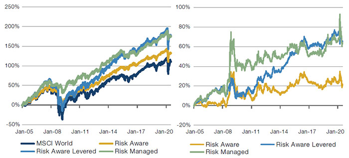
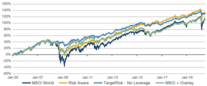
Table 6 quantifies the incremental benefit of each portfolio construction step to the performance and risk profile of the optimised risk-managed strategy. Performance is charted in Figure 12.

Table 6. Backtest Results

Source: Man Group, Bloomberg; between January 2005 and June 2020.
All metrics use end-of-month monthly returns except for 1M ES99, 1M ES95, and Skewness. These are calculated using 20-day overlapping returns.

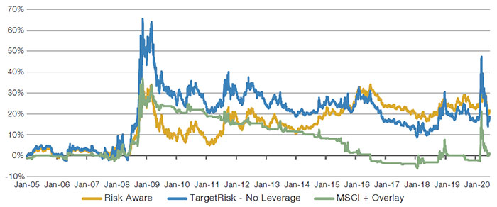
Figure 12. Compounded Returns (Log Scale, Left) & Difference from MSCI World Index (Right)

Simulated past performance is not indicative of future results. Returns may increase or decrease as a result of currency fluctuations.
Source: Man Group, Bloomberg; between January 2005 and June 2020.
Simulated performance data and hypothetical results are shown for illustrative purposes only, do not reflect actual trading results, have inherent limitations and should not be relied upon. Results are gross of any fees or expenses which could materially reduce returns. Please see the end of this paper for additional important information on simulated results.

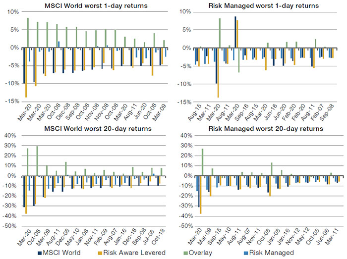
In Figure 13, we show the worst 1-day and 20-day returns for the MSCI World Index, the Risk Aware Levered portfolio and for the optimised risk-managed strategy. When the MSCI World Index experiences its worst returns, the Risk Aware Levered portfolio tends to experience similar negative returns, which is consistent with it having a beta close to 1. However, these times are also associated with strong performance for the risk overlays, so the optimised risk-managed strategy performs better than both the benchmark and the Risk Aware Portfolio. The worst return periods for the optimised risk-managed strategy typically coincide with periods when the risk overlays show little activity. The risk overlays are not a silver bullet. The optimised risk-managed strategy can still suffer tail events, but these are generally less frequent and less severe than those suffered by stocks portfolios without systematic risk management.

Sharp price corrections (or gap risks) remain a source of tail risk. Since the risk overlays generally react to changes in equity market conditions, they may not be in position at the time of a correction. (The exception here is the correlation overlay which anticipates when a bond sell-off can potentially spill over into equities.) Still, it is encouraging that the worst 1-day returns of the optimised risk- managed strategy are not large relative to the MSCI World Index, despite the use of leverage.

Figure 13. Worst MSCI and Risk-Managed Returns

Simulated past performance is not indicative of future results. Returns may increase or decrease as a result of currency fluctuations.
Source: Man Group, Bloomberg; between January 2005 and June 2020.
Simulated performance data and hypothetical results are shown for illustrative purposes only, do not reflect actual trading results, have inherent limitations and should not be relied upon. Results are gross of any fees or expenses which could materially reduce returns. Please see the end of this paper for additional important information on simulated results.

6. Conclusion

Using a combination of risk-based portfolio optimisation and dynamic risk-management, it is possible to construct an equity replacement strategy, which shows better risk-adjusted performance and tail characteristics than the MSCI World Index, with each portfolio construction steps providing incremental improvement. We believe that such a strategy can be a superior alternative to traditional global equity portfolios. Focusing on diversification in the core stocks holdings provides room to lever the portfolio during calm markets, capturing more of the equity risk premium than cap-weighted approaches, but with comparable risk. During periods of equity market stress, the addition of risk overlays reduces market exposure in the strategy below that of cap-weighted approaches: pulling the sails in until the storm passes.

7. Appendix: Exploiting the Modular Nature of the Strategy

One of the advantages of the framework described above is that it is highly flexible. This makes it easy to parametrise it to fit into the constraints different allocators might face. The following subsections provide examples of versions of the strategy where we change one or more parameters.

7.1. Changing Strategy Structure

The structure of the strategy is defined by several parameters. The two most important ones are:

• Leverage: is leverage allowed? If so, to what extent?;
• Short limits: is shorting allowed? If yes, to what extent? Is a short net position acceptable?

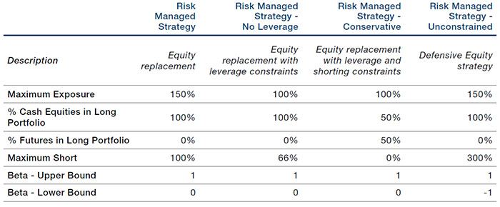
In this section, we provide simulations for a set of alternative structures. The point we want to highlight is this: while the constraints faced by different allocators might be varied, it’s usually possible to design a structure for the strategy to maintain the benefits of diversification and dynamic risk-management within the limits imposed by the allocator’s circumstances. We build a set of variations whose characteristics are explained in Table 7. In the tables and charts that follow, we present a summary of performance. In general, each of the strategies presents attractive risk-adjusted performance and tail characteristics, while respecting different constraints an allocator might face. This shows how the approach is flexible and able to improve outcomes also for investors with more restrictive requirements.

Table 7. Strategy Variations – Descriptions and Parameters

Source: Man Group. For illustrative purposes.

Table 8. Strategy Variations – Backtest Results

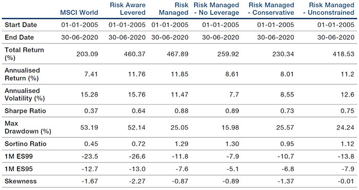
Source: Man Group, Bloomberg; between January 2005 and June 2020.
All metrics use end-of-month monthly returns except for 1M ES99, 1M ES95, and Skewness. These are calculated using 20-day overlapping returns.

Figure 14. Strategy Variations – Compounded Returns (log scale)

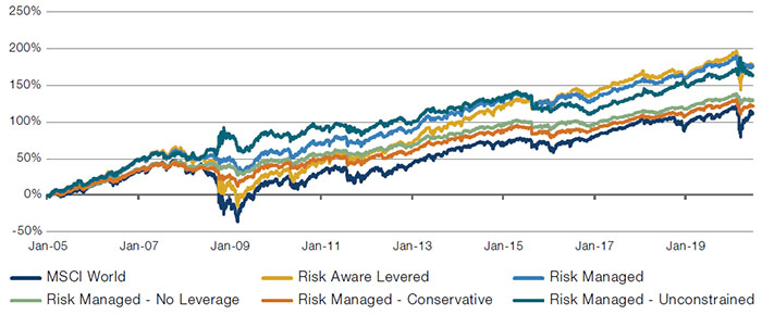
Simulated past performance is not indicative of future results. Returns may increase or decrease as a result of currency fluctuations.
Source: Man Group, Bloomberg; between January 2005 and June 2020.
Simulated performance data and hypothetical results are shown for illustrative purposes only, do not reflect actual trading results, have inherent limitations and should not be relied upon. Results are gross of any fees or expenses which could materially reduce returns. Please see the end of this paper for additional important information on simulated results.

Figure 15. Strategy Variations – Difference From MSCI World Index

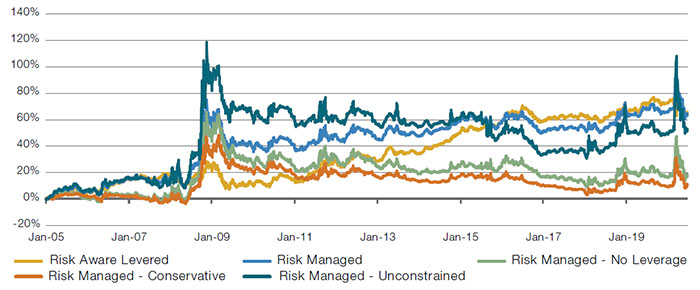
Source: Man Group, Bloomberg; between January 2005 and June 2020.

Figure 16. Strategy Variations – 20-Day Returns Correlations

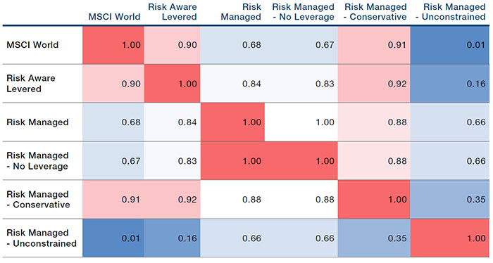
Source: Man Group, Bloomberg; between January 2005 and June 2020.

7.2. Changing the Benchmark: US-Focused Variation

The results outlined above also hold when we restrict the strategy to focus on a universe of US stocks. In this subsection, we use a universe of large US stocks for which the appropriate benchmark is the Russell 1000 Index. Table 9 shows that the process we followed in the Global universe still yields substantial improvements in performance when applied to the US universe. This could be an interesting variation for investors with a specific interest to the US market.

Table 9. US-Focused Variation – Backtest Results

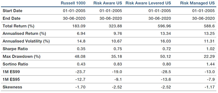
Source: Man Group, Bloomberg; between January 2005 and June 2020.
All metrics use end-of-month monthly returns except for 1M ES99, 1M ES95, and Skewness. These are calculated using 20-day overlapping returns.

Figure 17. US-Focused Variation − Compounded Returns (log scale)

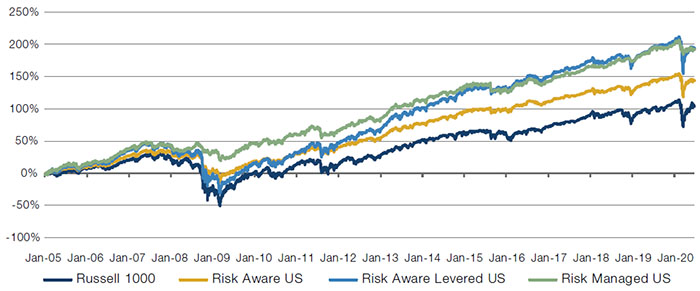
Simulated past performance is not indicative of future results. Returns may increase or decrease as a result of currency fluctuations.
Source: Man Group, Bloomberg; between January 2005 and June 2020.
Simulated performance data and hypothetical results are shown for illustrative purposes only, do not reflect actual trading results, have inherent limitations and should not be relied upon. Results are gross of any fees or expenses which could materially reduce returns. Please see the end of this paper for additional important information on simulated results.

Figure 18. US-Focused Variation – Difference from Russell 1000 Index

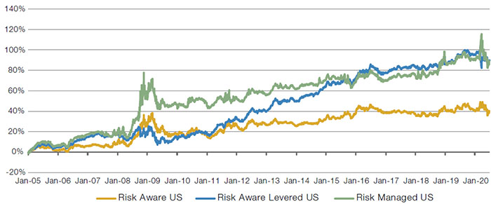
Source: Man Group, Bloomberg; between January 2005 and June 2020

7.3. Changing the Benchmark: EM-Focused Variation

In this section, we run an example similar to the one from the previous subsection. This time, however, we target the universe of emerging markets (‘EM’) stocks for which the appropriate benchmark is the MSCI Emerging Markets Index. Table 10 presents the futures we will use in the overlay, together with their allocations. We looked at the average allocations of the EM version of the Risk Aware portfolio over time and mapped them to index futures.

Table 10. EM-Focused Variation – Index Futures Allocations

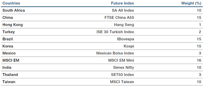
Source: Man Group; as of September 2020.

Table 11 presents data on the performance metrics and tail characteristics of the strategy. An important caveat is that for this variation we only have data since 2010. In general, we observe that the optimisation procedure we use to create the Risk Aware portfolio once again produces a portfolio with better risk-adjusted returns. The addition of the overlay does not have a meaningful impact on risk-adjusted performance for this time period, but still improves tail characteristics. Considering the short sample, we deem these results to be encouraging, as they go in the same direction as those we observed in the Global and US universe. We believe this strategy could be interesting for an allocator with a focus on EM equity markets.

Table 11. EM-Focused Variation – Backtest Results

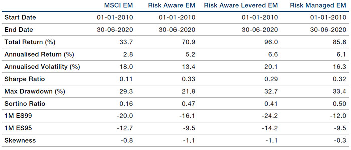
Source: Man Group, Bloomberg; between January 2010 and June 2020.
All metrics use end-of-month monthly returns except for 1M ES99, 1M ES95, and Skewness. These are calculated using 20-day overlapping returns.

Figure 19. EM-Focused Variation – Compounded Returns (log scale)

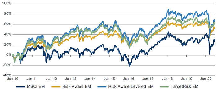
Simulated past performance is not indicative of future results. Returns may increase or decrease as a result of currency fluctuations.
Source: Man Group, Bloomberg; between January 2010 and June 2020.
Simulated performance data and hypothetical results are shown for illustrative purposes only, do not reflect actual trading results, have inherent limitations and should not be relied upon. Results are gross of any fees or expenses which could materially reduce returns. Please see the end of this paper for additional important information on simulated results.

Figure 20. EM-Focused Variation – Difference from MSCI EM Index

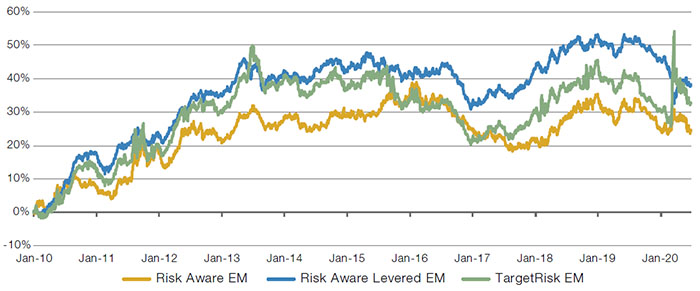
Source: Man Group, Bloomberg; between January 2010 and June 2020.

7.4. Applying the Overlay to a Pre-Existing Portfolio

In this section, we look at the effect of applying the short overlay to a pre-existing portfolio, mirroring the composition of the MSCI World Index. This could be a solution for an investor who does not want to deviate from an already-existing allocation to global equity markets, but who is interested in a defensive strategy that will protect the portfolio in times of stress. Table 12 shows a summary of performance and tail characteristics for this variation when compared to the optimised Risk-Managed – No Leverage variation from Section 7.1, where we do not allow leverage. Adding the Overlay to the MSCI World Index produces an improvement in risk-adjusted performance and tail characteristics (skewness, max drawdown, expected shortfall). This enhanced MSCI World portfolio is still inferior to the comparable optimised risk-managed strategy variation, which has even better risk-adjusted performance and tail characteristics. However, if this is not a viable option, deploying just the overlay could still lead to improved outcomes.

Table 12. Overlay on Pre-Existing Portfolio – Performance

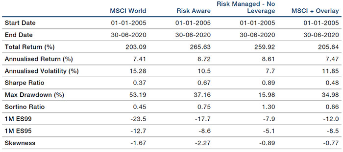
Source: Man Group, Bloomberg; between January 2005 and June 2020.
All metrics use end-of-month monthly returns except for 1M ES99, 1M ES95, and Skewness. These are calculated using 20-day overlapping returns.

Figure 21. Overlay on Pre-Existing Portfolio – Compounded Returns (log scale)

Simulated past performance is not indicative of future results. Returns may increase or decrease as a result of currency fluctuations.
Source: Man Group, Bloomberg; between January 2005 and June 2020.
Simulated performance data and hypothetical results are shown for illustrative purposes only, do not reflect actual trading results, have inherent limitations and should not be relied upon. Results are gross of any fees or expenses which could materially reduce returns. Please see the end of this paper for additional important information on simulated results.

Figure 22. Overlay on Pre-Existing Portfolio – Difference From MSCI World Index

Source: Man Group, Bloomberg; between January 2005 and June 2020.

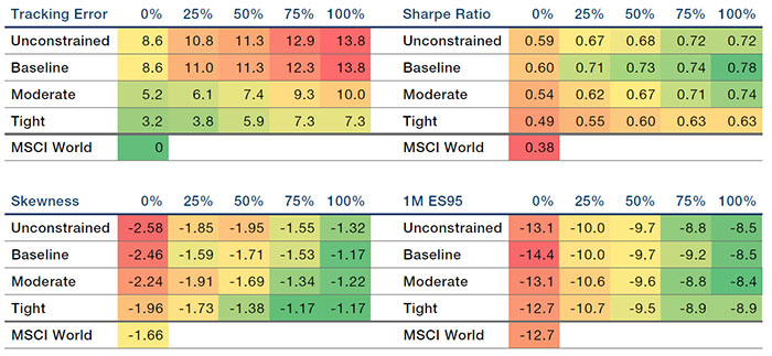
7.5. Managing Tracking Error

In this section, we look at ways to control the tracking error of the portfolio against a benchmark. Tracking error considerations might be important for a client who wants control over the deviation from a reference index. There are two main ways of achieving this goal: (i) optimise the cash equity portfolio subject to a tracking error constraint; and (ii) reduce the maximum short position taken by the futures overlay. We will examine different combinations of the two solutions.

As a first step, we build a set of baseline cash equity portfolios with different tracking error constraints.⁸ The portfolios differ across three main areas:

• They use different tracking error penalties in their objective function. The higher the penalty the lower the tracking error;
• They have different industry/region constraints against the benchmark. The more relaxed the constraints the higher the tracking error;
• They have different beta constraints. The tighter the beta constraint the lower the tracking error.

As a second step, we apply overlays with different maximum short positions to the baseline cash portfolios. The larger the maximum short, the higher the tracking error.

In Figure 23, we look at the summary statistics of different combinations:

• We use four baseline cash portfolios: a ‘Baseline’ version, which is similar to what we used in the rest of this note in terms of constraints, an ‘Unconstrained’ version, and two versions with ‘Moderate’ and ‘Tight’ constraints;
• We apply five different levels of maximum overlay short: from 0% (no overlay) to 100% of capital in increments of 25%.

Figure 23. Summary Statistics – Different Combinations of Baseline Portfolio and Maximum Overlay Short

Simulated past performance is not indicative of future results. Returns may increase or decrease as a result of currency fluctuations.
Source: Man Group, Bloomberg; between January 2005 and June 2020.
Simulated performance data and hypothetical results are shown for illustrative purposes only, do not reflect actual trading results, have inherent limitations and should not be relied upon. Results are gross of any fees or expenses which could materially reduce returns. Please see the end of this paper for additional important information on simulated results.

We note that both portfolio construction and the amount of the overlay we use contribute similarly to tracking error. None has a dominant effect. As for tail properties instead, these are mainly determined by the amount of the overlay we allow. The more constrained portfolios show marginally better properties, but there is no specific reason why this should be expected to continue in the future, as constraints don’t have as an objective that of improving tail properties. In general, if we want to reduce tracking error the right choice will probably be in the middle: both running a more constrained portfolio and reducing the maximum short in the overlay.

In Figure 24, we visualise the trade-off between tracking error and performance. The relationship between Sharpe ratio and tracking error is approximately linear. A tracking error constraint can be represented as a vertical line on the chart. To reiterate: a conservative approach to reduce tracking error will most likely achieve the objective by both running a more constrained portfolio and by reducing the size of the overlay.

Figure 24. Summary Statistics Versus Tracking Error – Different Combinations of Baseline Portfolio and Maximum Overlay Short

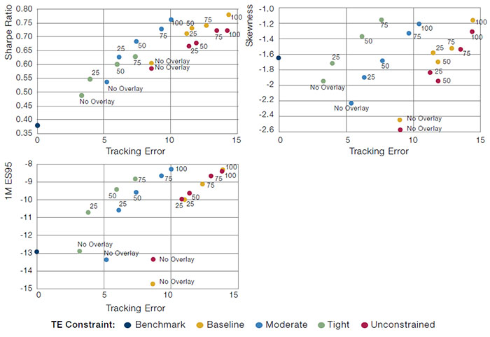
Simulated past performance is not indicative of future results. Returns may increase or decrease as a result of currency fluctuations.
Source: Man Group, Bloomberg; between January 2005 and June 2020.
Simulated performance data and hypothetical results are shown for illustrative purposes only, do not reflect actual trading results, have inherent limitations and should not be relied upon. Results are gross of any fees or expenses which could materially reduce returns. Please see the end of this paper for additional important information on simulated results.

1. See for example: The Impact of Volatility Targeting.
2. F. Black, M. Jensen and M. Scholes, The capital asset pricing model: some empirical tests. In M. Jensen, ed.: Studies in the theory of capital markets (Praeger), 1972.
3. F. Black. Capital market equilibrium with restricted borrowing. Journal of Business, 45(3):444–455, 1972.
4. We follow a simplified methodology to build these portfolios rather than the complete procedure we will use in the rest of the text. The characteristics of the resulting portfolios remain similar to what used in the rest of the text.
5. In performance tables, we refer to the 99% (95%) Expected Shortfall of 1-month returns as 1M ES99 (1M ES95).
6. In our backtests, we assumed a financing cost of 25 bps over 3-Month US LIBOR.
7. Skewness is a measure of the asymmetry in the distribution of returns. Loosely speaking, negative skewness indicates that a bad daily loss is larger than a good daily gain.
8. We follow a simplified methodology to build these portfolios rather than the complete procedure covered in the main body of the text. The characteristics of the resulting portfolios remain similar to what used in the main text.

Hypothetical Results

Hypothetical Results are calculated in hindsight, invariably show positive rates of return, and are subject to various modelling assumptions, statistical variances and interpretational differences. No representation is made as to the reasonableness or accuracy of the calculations or assumptions made or that all assumptions used in achieving the results have been utilized equally or appropriately, or that other assumptions should not have been used or would have been more accurate or representative. Changes in the assumptions would have a material impact on the Hypothetical Results and other statistical information based on the Hypothetical Results.

The Hypothetical Results have other inherent limitations, some of which are described below. They do not involve financial risk or reflect actual trading by an Investment Product, and therefore do not reflect the impact that economic and market factors, including concentration, lack of liquidity or market disruptions, regulatory (including tax) and other conditions then in existence may have on investment decisions for an Investment Product. In addition, the ability to withstand losses or to adhere to a particular trading program in spite of trading losses are material points which can also adversely affect actual trading results. Since trades have not actually been executed, Hypothetical Results may have under or over compensated for the impact, if any, of certain market factors. There are frequently sharp differences between the Hypothetical Results and the actual results of an Investment Product. No assurance can be given that market, economic or other factors may not cause the Investment Manager to make modifications to the strategies over time. There also may be a material difference between the amount of an Investment Product’s assets at any time and the amount of the assets assumed in the Hypothetical Results, which difference may have an impact on the management of an Investment Product. Hypothetical Results should not be relied on, and the results presented in no way reflect skill of the investment manager. A decision to invest in an Investment Product should not be based on the Hypothetical Results.

No representation is made that an Investment Product’s performance would have been the same as the Hypothetical Results had an Investment Product been in existence during such time or that such investment strategy will be maintained substantially the same in the future; the Investment Manager may choose to implement changes to the strategies, make different investments or have an Investment Product invest in other investments not reflected in the Hypothetical Results or vice versa. To the extent there are any material differences between the Investment Manager’s management of an Investment Product and the investment strategy as reflected in the Hypothetical Results, the Hypothetical Results will no longer be as representative, and their illustration value will decrease substantially. No representation is made that an Investment Product will or is likely to achieve its objectives or results comparable to those shown, including the Hypothetical Results, or will make any profit or will be able to avoid incurring substantial losses. Past performance is not indicative of future results and simulated results in no way reflect upon the manager’s skill or ability.