Reasons to Stick with Commodities, Even If Inflation Eases

Summary

In this inflation surge, commodities have been the star performer, while traditional assets like equities and bonds have faltered. Now that inflation is close to peaking, should asset allocators persist with their commodities allocation? We argue that, despite inflation peaking, there are still significant positives: commodities provide quite unique diversification benefits, are only in Year 2 of a multi-year bull market driven by lack of supply, positioning is light, and the curve is in backwardation.

Commodities are a crucial part of multi-asset portfolios

This is even more true if indeed we enter a prolonged period of high and volatile inflation, as per our expectation. This was the strong conclusion from our paper The Best Strategies for Inflationary Times, in which we showed that a diversified basket of commodities had a 100% hit rate of delivering positive real return during inflationary surges, in the last 100 years.¹

Furthermore, they provide attractive diversification benefits, albeit least in period of deflation. The case for commodities is not only contingent on a view to expect high and volatile inflation. Diversification is the most important feature of portfolio management, and commodities provide heaps of it.

Commodities are least diversifying in periods of Deflation (aka Ice in our Fire & Ice framework, shown in Figure 1), and most diversifying in periods of Inflation (aka Fire). In Disinflation, historically, commodities have been very diversifying, too. Figure 7 (see Appendix) shows that the average correlation between commodities and equities and bonds is 0.24 and -0.08, respectively.

Figure 1. The Fire & Ice Framework

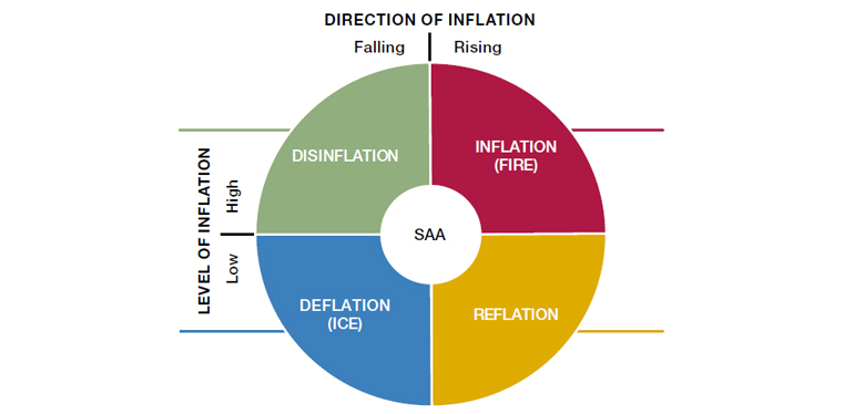
Source: Man Solutions.

Commodities have provided positive return through time

We find that our diversified backet of commodities has returned 4% annualised real over time. This finding is consistent with other studies such as ‘Commodities for the Long Run’ (Levine et al., 2018) and those reported in chapter 4 of Antti Ilmanen’s ‘Investing Amid Low Expected Returns’ (2022). It is interesting to note, in passing, that without regular rebalancing this return is lower, as individual commodities typically compound lower returns over time.

There are considerable variations in commodities’ return by economic regime, with the best results during Inflation, and the worst in Deflation. Figure 8 (see Appendix) shows that a diversified basket of commodities has delivered +14% annualised real in Inflation, +7% in Reflation, 0% in Disinflation, and -13% in Deflation. This offers a nice skew. For long-term investors, Commodities carry little downside and potentially a lot of upside, unless the rare Deflation quadrant is in play – this quadrant has occurred only 7% of times historically and is an unlikely scenario at this stage, in our view.

A Strategic Asset Allocation (“SAA”) of 4.5% in a hypothetical multi-asset portfolio

The above considerations naturally feed a strategic allocation to commodities in each of the four Fire & Ice regimes. Let’s take a hypothetical portfolio with as starting point an SAA of equal risk contribution from Equities, Bonds and Alternatives, and commodities being one of the Alternatives strategies. For sizing we use our method of “clustered expected tail loss”. This method is a close cousin of volatility scaling, but now focussed on volatility in the left tail so as to minimise the risk of significant losses at the portfolio level. Without going into the details, which include sizing allocations such that the portfolio achieves 6-8% vol at the aggregate level, we calculate the optimal SAA to commodities is 4.5% if one is agnostic about the current F&I regime.

However, this optimal SAA can be as high as 9% in Inflation, and as low as 1% in Deflation. We calculate that the optimal allocation can be as high as 9% in Inflation, 7% in Reflation, and 1% in both Disinflation and Deflation, still within the context of the aforementioned hypothetical multi-asst portfolio.²

Tactical Asset Allocation (“TAA”) considerations

Even we would admit that there is more to an investor’s life than Fire & Ice. Additional angles of analysis can improve asset allocation decisions. These include the following, and are all pointing in a positive direction for commodities, currently, in our view:

1. Fundamental historical analysis shows multi-year bull and bear cycles for commodities, driven by long lead times in supply: Due to the long lead cycles for supply, commodities in and of themselves – as well as their relative performance versus equities -- follow a pattern of multi-year markets (more detail on this point can be found in Jim Rogers’ (2000) Hot Commodities). Historically, most often, the bull and bear cycles have lasted over a decade. Figure 2 suggests the average cycle for commodities in isolation is 12 years. Figure 3 implies a normal commodities-versus-equities regime is 16 years long. Mining specialists we speak to argue that the supply bottlenecks and lead times have worsened for regulatory reasons, as well. Currently it seems clear to us that commodities are only in year two of a bull market which, if historical precedent is any guide, may last a decade or more.

Figure 2. The Persistence of Historic Commodities Bull and Bear Markets

Problems loading this infographic? - Please click here

Source: Man Solutions; as of September 2022. Chart shows the trailing 10Y nominal CAGR for the equal weight commodity basket and has been optically divided into bull and bear markets (bear markets shown in red). Numbers at the top indicate the length of each of these episodes.

Figure 3. The Persistence of Historic Commodities Versus Stock Returns

Problems loading this infographic? - Please click here

Source: Man Solutions. Chart indexes the commodity and equity prices at 100 in February 1877 then each month divides the commodity index by the equity index, then takes the log(10) of the result. The series is divided optically into bull and bear markets (bear markets shown in red) and the numbers at the top indicate the length of each of these episodes.

2. Shorter-term considerations, such as consensus positioning. For more short-term trading considerations, one can track technical developments such as momentum; distance from moving averages; commodities’ FX levels compared to the underlying commodity price; and CFTC positioning to assess sentiment, with extreme bullish or extreme bearish positioning an early warning signal for a turning point. Figure 4 shows excessive negative positioning on our commodities aggregate, which we consider as a positive, all things equal.

Figure 4. Commodities Not Quite So Popular Anymore Among Speculators

Problems loading this infographic? - Please click here

Source: Man Solutions; as of September 2022. For each of oil, natural gas, copper and gold, we take the CFTC net non-commercial combined position as a % of total open interest. We then transform this into a 3 year z score. We then weight each of these components, respectively, at 31%, 20%, 23% and 27%, being their approximate weighting within the BBUXALC index. Prior to 2010, there is no CFTC natural gas data and thus prior to then we proxy natural gas with oil.

3. Last but certainly not least, there is the very important information contained in the shape of the futures curve. Commodity returns have a spot as well as a roll or carry component. The return from the spot component, naturally, stems from changes in price of the physical commodity. The roll or carry component is the return from investing in the liquid future – typically front month -- and the return from the price change in the future as a result of the future converging with the spot price if held to maturity. Historically this roll has generated positive returns of around 5% per annum, per The Commodity Futures Risk Premium: 1871-2018 by Bhardway et al.

Historically, commodity futures perform best when the curve is in backwardation. If the forward curve in in backwardation, it means that the price of the future contract is lower than the spot price, hence the roll is expected to be positive. Various studies have quantified this effect. Bhardway et al (2018) confirm that the commodity risk premium has equalled 11% when the curve is in backwardation, versus only 1% when the curve is in contango. The logical conclusion to buy the future when the curve is in backwardation can be further empirically supported by work published in 2018 in ‘Commodities for the Long Run’. Figure 5 shows that commodity mean return (roll + spot) equalled 4.6% through time: 7.7% when the curve was in backwardation and 1.8% when in contango. The roll return is much higher when the curve is in backwardation. The spot return is somewhat lower when the curve is in backwardation, but the roll+spot return is highest in backwardation.

Figure 5. Commodities Returns are Best When the Curve is in Backwardation

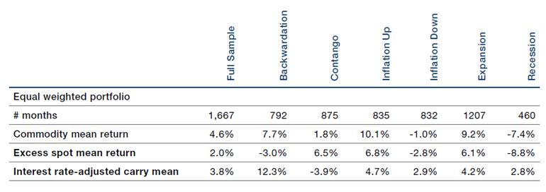
Source: Levine et al. (2018) Commodities for the Long Run. Expansion is trough to peak based on NBER dating, and recession is peak to trough based on NBER dating. Aggregate backwardation/contango states for the long–short portfolio are based on aggregate states for the equal-weighted index. Commodity futures index returns do not equal the sum of excess spot returns and interest rate–adjusted carry because of the cross-term.

Figure 6 shows our aggregate forward curve proxy for our favourite commodities aggregate. We conclude that currently the forward curve is implying a positive carry and therefore is giving a positive trade signal, ceteris paribus.

Figure 6. The Curve Currently Is in Backwardation - A Positive Signal

Problems loading this infographic? - Please click here

Source: Man Solutions; as of September 2022. Proxy shown is calculated for BBUXALC. For each of oil, natural gas, copper and gold, we calculate the shape of the futures curve as a % of the spot at the respective time. We then weight each of these components, respectively, at 31%, 20%, 23% and 27%, being their approximate weighting within the BBUXALC index. The ‘Typical Curve’ is calculated as the average of the curves in September of 2021, 2020, 2019, 2018, 2017, 2016 and 2015.

Conclusion: we find strong reasons to stick with a healthy allocation to commodities despite easing inflation

Where does that leave us for our commodity investment within the hypothetical multi-asset portfolio? All in all, if the correct allocation to Commodities was 9% in Inflation, we think the allocation from here on should be lower but a still healthy 4%. This is a higher number than the 1% implied by our SAA analysis in Disinflation. We get to this conclusion because of our judgment that a) commodities are in the early stages of a long bull market; b) positioning is low not high; and c) the implied carry by the forward curve is currently positive. In Disinflations, Commodities still provide diversification, indeed on average in this episode through history, the correlation between commodities and a US 60/40 portfolio has been a relatively low 0.16 (Figure 7). While the average return has been 0% in this Fire & Ice quadrant, we believe the likelihood is that returns will outstrip this average, in addition to the diversification benefits.

Appendix

Figure 7. Commodities provide heaps of diversification

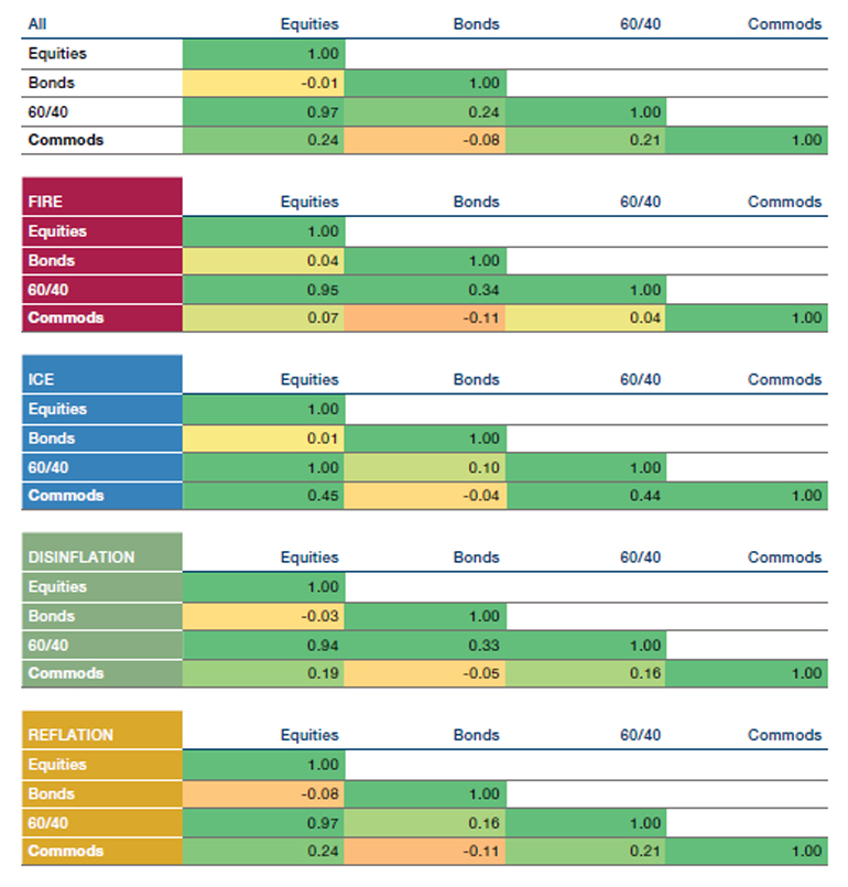
Source: Man Solutions; as of September 2022. Colours range from -0.3 (green) through 0 (yellow) to +0.3 (red). Data from 1926 to June 2022. Equities are proxied by S&P 500 from Professor Shiller’s database. Bonds are UST10. 60/40 is the combination of the two, monthly rebalanced. Commodities use AQR series up until 1946 and then Man Group’s own archived data since then. The commodities basket is made up of near end futures, equal weighted across commodity groupings.

Figure 8. Commodities Returns Vary by Economic Regime – Inflation Best, Deflation worst

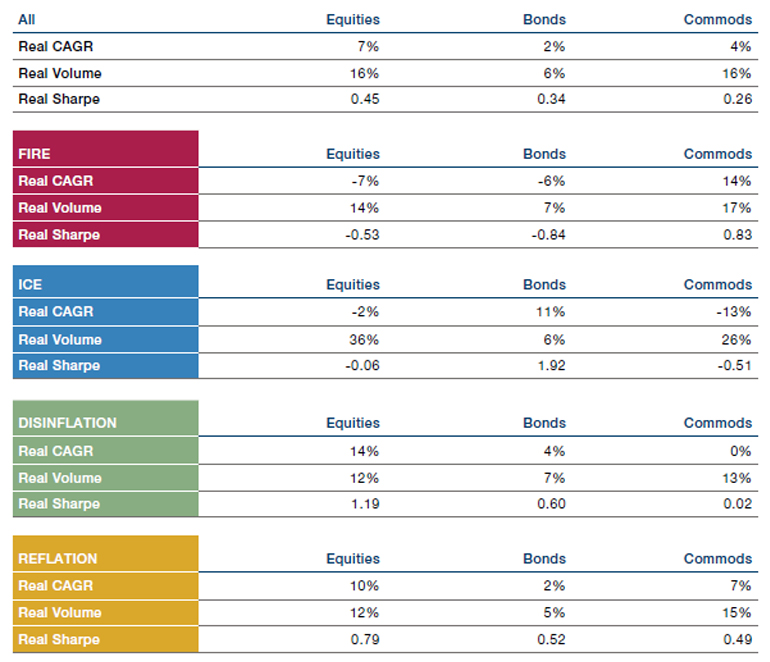
Source: Data from 1926 to June 2022. Equities are proxied by S&P 500 from Professor Shiller’s database. Bonds are UST10. 60/40 is the combination of the two, monthly rebalanced. Commodities use AQR series up until 1946 and then Man Group’s own archived data since then. The commodities basket is made up of near end futures, equal weighted across commodity groupings.

1. GSCI (with data since 1970), BCOM (since 1960) and BBUXALC (since 1991) are the three most important commodity indices. In this piece, for current analysis, we focus on BBUXALC – the UCITS-compliant Bloomberg Commodity ex Agriculture and Livestock Capped financial index. In our historical analysis we used our own extensive database to create an index with more history. To be precise, we use the average return for the following 6 groups: industrials (copper), precious (gold, silver, palladium), agris (wheat, corn, soybeans), softs (cocoa, cotton, coffee, sugar), livestock (cattle, hogs), energies (Brent, WTI, heating oil). Nominal returns are funded, in other words the return of the contract plus the risk-free rate as reported by the Kenneth French website. The real returns are the funded returns, minus inflation. The strategies take whichever futures contract is most liquid within the Man AHL database. This is not always the first month but will be in the early part of the curve. Returns are equally weighted averages, month by month. Where one commodity in the group is not available, the average of the others is taken. The “Commodity Aggregate” category is a month-by-month, equally weighted average of the aforementioned commodity groups. All returns are in USD.
2. Please note that these sizing considerations refer to a long-only allocation to a diversified commodities basket in the context of this hypothetical portfolio. In addition, a multi-asset portfolio can benefit from dynamic strategies that allocate to commodities and other asset classes in a risk-controlled manner, for instance based on automated alpha signals related to price momentum or economic regime. We do not consider such strategies in this exercise.