Key takeaways:
- History has shown us that investors who shoulder higher risk over the long term are compensated by higher expected returns. Yet the short-run relationship between risk and returns is not straightforward and not all investors can tolerate mark-to-market losses
- While there is a large amount of randomness in financial markets, particularly in relation to the direction of returns, some other features of market prices are more predictable, namely risk and diversification
- Drawing on our experience managing systematic hedge funds, which we have accumulated over more than 35 years, we outline how predictability can help long-only investors to improve risk-adjusted returns without the need to forecast the direction of returns
Introduction
The volatility we witnessed at the beginning of August was a sharp reminder that shocks can hit markets suddenly and sometimes without a clear driver. Navigating periods of market turbulence is an unavoidable feature of long-term investing. We know of two effective approaches to this. The first is to be passive: soak up the volatility and potential drawdowns and bet on growth in the long run. That’s all well and good for those who have the luxury of being able to ignore mark-to-market losses, but that’s not the majority. Further, drawdowns can have consequences for the ongoing operations of endowments, pension funds, and the like.
The second option is to take a risk-based approach to investing: build a diversified multi-asset portfolio and actively manage risk. Diversifying across asset classes can build robustness to economic shocks, and active risk management can insulate against periods of market stress or volatility. It is this diversifying, active approach that we focus on in this paper. We begin by considering in more detail the challenge that investors face in navigating volatile markets and demonstrate how taking a risk-based approach to investing can improve diversification and ultimately enhance risk-adjusted returns.
The challenge investors face
Asset prices are continuously being buffeted by economic, financial and geopolitical shocks. Anticipating changing market trends is challenging. At the same time, some patient, long-term investors have been able to profit from holding risky assets – either explicitly or implicitly sharing in the wealth created by economic activity.
However, Figure 1, which takes a long view of US stock market data, demonstrates how the level of market risk has varied significantly through time. The average volatility in the US stock market has been just short of 15% since 1927 yet in the first quarter of 2020, at the start of the Covid-19 pandemic, market volatility was over 50%. The amount of return variation experienced in that single quarter was equivalent to two-and-a-half average years. Most of the quarters with very high return variation are demarked with red bars, indicating that high volatility is generally coincident with falling markets: the so-called leverage effect.
Figure 1. Variation of US stock market returns and volatility
The top panel shows daily stock market returns in excess of Treasury bills. The middle panel shows the annualised volatility of returns. The bottom panel expresses quarterly return variation in terms of mean annual return variation (e.g. a value of two indicates that two years of average variation was experienced in a single quarter). Bars are coloured green or red depending on whether stock returns (excess of bills) were positive or negative over the quarter. So in the top panel all bars in a quarter are red if the return over the quarter was negative, whereas in the middle and bottom panels there is a single green or red bar per quarter.
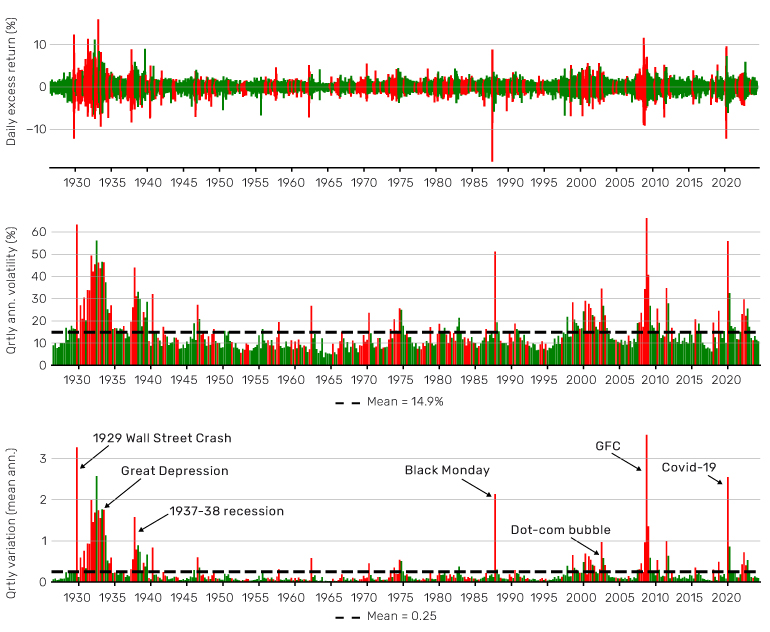
Source: Kenneth French, Man Group. Data from July 1927 to June 2024.
So, stocks are risky. This will not be news to many. In the long run, particularly in the US, the stock market has delivered real returns far outstripping cash or bonds (Hoyle, 2020). This is in keeping with the theory that investors who shoulder higher risk are compensated by higher expected returns. We do not dispute this long-run relationship. However, the short-run relationship between risk and returns does not fit this pattern. We shall return to this shortly and show how we can use it to our advantage.
Diversification: a powerful ally
In the meantime, let’s briefly consider diversification, a well-known and powerful ally in portfolio construction. A diversified portfolio is one where the overall portfolio risk is well spread across individual sources of risk. Typically, traded instruments or asset classes are viewed as the sources of risk. Let’s take, for example, the risk of bonds versus equities. In a diversified multi-asset portfolio, we should expect the equities risk to be comparable with bonds risk.
In addition, we can consider macroeconomic shocks as sources of risk. There are compelling macroeconomic arguments for diversifying across asset classes. For example, the level and direction of inflation in the US provide useful discriminants for the historical performance of asset classes. We demonstrate this in Figure 2, which we reproduce from (Neville, Draaisma, & Funnell, 2022). The two regimes that stand out as negative for equities are ‘fire’ (high and rising inflation) and ‘ice’ (low and falling inflation). During periods of fire, commodities have historically performed well since they are real assets. During periods of ice, bonds have performed well as the present value of fixed coupons has increased in value. Diversification across asset classes can insulate portfolios against macroeconomic risks. In particular, adding bonds and commodities can provide a buffer during regimes that are unfavourable to equities.
Figure 2. Performance of US assets by macroeconomic regime (real, annualised returns)
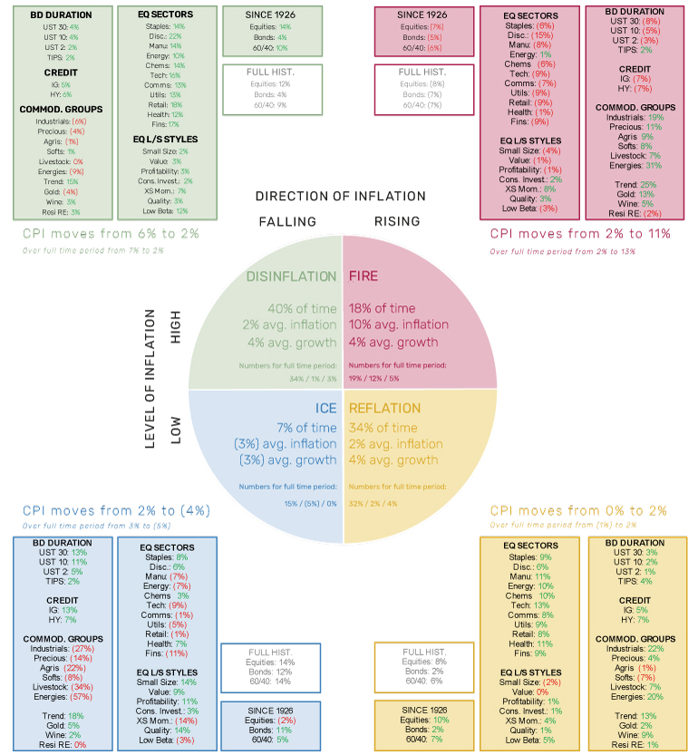
Source: Reproduced from (Neville, Draaisma, & Funnell, 2022). Covers period from 1877 to 2022. For further details on regimes and asset returns, please see (Neville, Draaisma, Funnell, Harvey, & Van Hemert, The Best Strategies for Inflationary Times, 2021). Source: Robert Shiller, Kenneth French, GFD, AQR, Golman Sachs, Bloomberg, Morgan Stanley, Credit Suisse, Liv-ex, Man Group.
Improving returns by forecasting risk
Turning now to risk, a simple measure of risk-adjusted returns is to divide returns by volatility (R/σ). There are two mechanisms to increase risk-adjusted returns: (i) target the numerator R: take more exposure when returns are higher and less when returns are lower, or (ii) target the denominator σ: take less exposure when volatility is higher and more when volatility is lower. In either case, forecasting is required since we need to predict whether returns or volatility will be higher or lower. Forecasting the direction of returns accurately is notoriously difficult, but it is possible to forecast volatility. Figure 3, inspired by (Harvey, et al., 2018), demonstrates this. It compares the monthly return and volatility (risk) of US stocks to the volatility realised in the prior month. By calendar month, market volatility has generally been higher if the previous month was volatile. Notice also that returns were not generally higher if market risk was higher, as we alluded to earlier. What can we conclude from this? After a period of higher volatility, we should expect continued higher volatility, but not commensurately higher returns. In the short term then, investors are not rewarded for bearing higher risk.
The persistence (or clustering) of volatility is one of the most pervasive features of asset prices and can been seen across asset classes. In Figure 4, for a large range of liquid instruments, we show that there is little autocorrelation in calendar month returns, but there is high autocorrelation in the variance of returns. So past returns are not a strong predictor of future returns, but past risk can be a strong predictor of future risk.
Let’s return to our two methods of improving risk-adjusted returns outlined at the beginning of this section. We have seen that neither past volatility nor past returns give much insight into future returns. So, let’s assume that expected returns are constant. We have seen that past volatility is a good predictor of future volatility. Using past volatility as a risk forecast, we can take more exposure in low volatility environments and less exposure in high volatility environments to target higher risk-adjusted returns.1
As a final note on forecasting, cross-asset correlations are an important driver of risk in multi-asset portfolios. Figure 5 shows that the bond-equity correlation is highly variable, but it is also persistent. Historically, periods of negative (resp. positive) correlation have typically been followed by periods of negative (resp. positive) correlation. So we can use recent cross-asset correlations to forecast futures correlations.
Figure 3. Calendar-month mean excess return and realised volatility by quintile of prior month return volatility for US stocks
There is no clear pattern between prior month volatility and subsequent returns. In the short-run, investors have not clearly been rewarded for holding stocks after periods of high volatility. However, there is a clear, positive relationship between stock volatility in a calendar month and the volatility in the prior month.
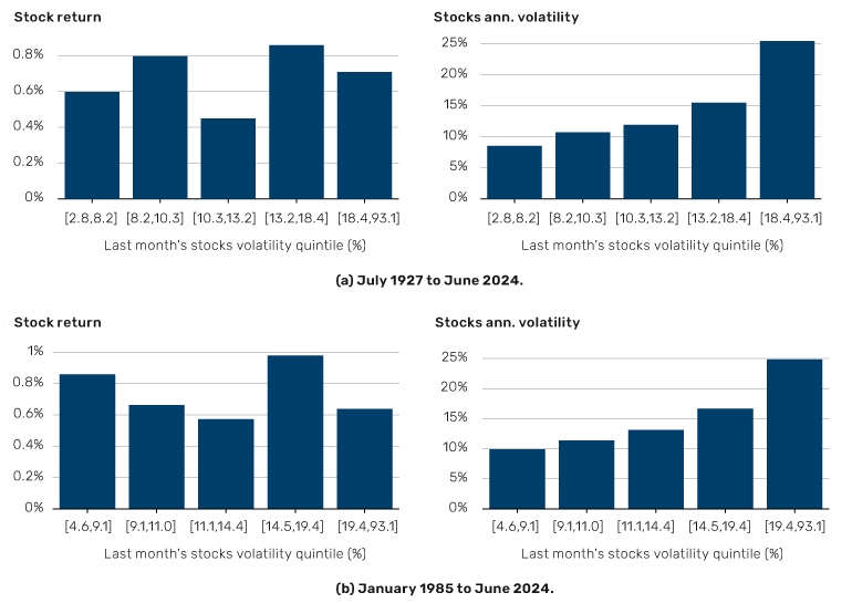
Source: Kenneth French, Man Group. Time periods selected based on availability of reliable data.
Problems loading this infographic? - Please click here
Problems loading this infographic? - Please click here
Taking an active approach to risk management
Let’s turn now to risk management, an important feature of any portfolio management process. A traditional approach is to be reactive: risk managers or portfolio managers make changes to a portfolio if its risk becomes unacceptably high. In these cases, reactive risk management is exogenous to the investment process.
Active risk management describes an alternative approach whereby risk controls are incorporated into the investment process. This does not necessarily replace reactive risk management, but – employed effectively – it can reduce the frequency of reactive interventions. Systematic investment is particularly suited to the application of active risk management, which includes volatility targeting (sizing positions inversely proportional to volatility, see [Harvey, et al., 2018]) as well as the application of tail-risk mitigations that reduce exposure during times of market stress.
Dynamic risk targeting
We must remember that high risk-adjusted returns do not necessarily translate into high returns. If the overall level of risk is very low, then a small positive return may translate into a high risk-adjusted return. Over the longer term we do not dispute finance theory: to achieve higher returns you must be prepared to bear higher risk. If possible, we should avoid asset class allocation as a tool to reach our appropriate risk level (e.g. more equities and less bonds for more risk).
Instead, we should balance risk across asset classes, and then follow (Tobin, 1958) by allocating between the balanced portfolio and a minimal risk portfolio (e.g. of government bills) according to our risk preference. We may need to lever our balanced portfolio to attain our required level of risk. Unless the cost of leverage is high, this is reasonable, sensible even, use of leverage to build a diversified portfolio. This could hardly be further from the use of leverage to take highly concentrated bets, the type of behaviour that gives leverage a bad name.
With that said, we also recognise that future diversification can never be known with certainty. Correlations between asset classes vary through time. In times of market stress, correlations can change quickly. So, users of leverage must remain vigilant and may have to react to changing market conditions.
We now demonstrate how taking a risk-based approach to investing can improve diversification and manage portfolio risk. For exposition, we focus on a two-asset problem of investing in US equities and bonds but note that the principles generalise more broadly, including to commodities. The 60/40 portfolio allocates 60% of capital to equities and 40% to bonds. On the face of it, this sounds diversified. However, much more than 60% of the risk in the portfolio is allocated to equities. In the long run, more than 80% of the risk is in equities, with this rising above 90% in periods of market stress. The diversification is skin deep. The volatility of equities and bonds, and their correlation, are highly variable, leading to high variability in the volatility of the 60/40 portfolio. But as we have seen, these volatilities and correlations are persistent, and so we can forecast them with greater accuracy. We can produce a simple risk-managed variation of the 60/40 portfolio that targets a 60% risk allocation to equities and a portfolio annualised volatility of 11%, which is similar to the longrun volatility of the 60/40 portfolio. The risk targeting is based on scaling positions inversely to recent volatility (exponentially weighted volatility with a half-life of 65 days). Figure 6 compares some of the risk characteristics of the 60/40 portfolio and our risk-managed version. Here are some key observations:
- In the more traditional 60/40 approach, equities contribute around 80% of the risk, but this can vary greatly from year to year. In the risk-managed approach, we reduce the target equity risk contribution to 60% to improve diversification. Not only is this diversification achieved in the long run, but also the risk contribution is tightly controlled around the target 60%
- In the more traditional approach, portfolio risk varies widely around a long run value 11% annualised volatility. With risk management, the volatility of the portfolio is tightly controlled to its 11% volatility target. Importantly, improving the diversification in the portfolio has not led to a reduction in risk taking
Figure 6. Risk characteristics of US equities and bonds portfolios
‘60/40’ targets a 60% exposure to equities and 40% bonds. ‘Risk managed’ uses recent realised volatility (exponentially weighted with 65-day half-life) to rebalance daily to 60% equity risk and 40% bond risk, and to target a portfolio volatility of 11% (to match 60/40). In the left panel, equity risk contribution is the rolling 260-day standard deviation of equity returns divided by the sum of the rolling 260-day standard deviations of equity and bond returns. In the right panel, portfolio volatility is the rolling 260-day standard deviation of returns.
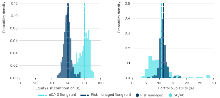
Source: Man Group. Based on S&P 500 and US 10-year note futures from January 1985 to June 2024. Time period selected based on availability of reliable data.
In our risk-managed portfolio, we are controlling for two effects: the changing volatilities of equities and bonds, and the changing correlation between equities and bonds. In a static portfolio, the amount of diversification achieved through time will vary according to market conditions.
Mitigating tail risks
During market crises, previously hidden tail dependencies tend to reveal themselves and it is not prudent to depend on long-term or even medium-term levels of diversification. Cross-asset correlations can increase quickly in a broad sell-off, increasing portfolio risk. In these cases, a more aggressive approach to managing risk may be required. There are two steps involved here. The first is to identify signs of market stress in real time. The second is to adjust positioning quickly and efficiently in response.
There are many data-driven ways to identify market stress. When looking for signs, we prefer to focus on financial data. Economic data are important, but are often released at low frequency, with reporting lags and subject to significant revision. These data can be helpful for contextualising past episodes but are less suited to real-time monitoring. Price data for liquid assets, on the other hand, are available at high frequency, with minimal lags, and are rarely revised. Asset prices are also inherently forward-looking, reflecting market views of the size and reliability of future cash flows. There are various features of prices that can act as warning signs.
Among the measures we like to monitor are asset price momentum, volatility spikes and cross-asset correlations. Price momentum helps identify and reduce exposure to markets in freefall. A spike in volatility across an asset class can be an early indicator of crisis, particularly in risk assets. A spike in volatility across a multi-asset portfolio may reflect higher cross-asset correlations, and a loss of diversification. Cross-asset correlations can also be monitored directly. More subtle features may include jointly monitoring cross-asset correlations and price trends, looking for signs of contagion. Correlations alone can provide some insight into the key macroeconomic risks driving markets. For example, we would expect to see higher stock-bond correlations when inflation risk dominates growth risk, and lower correlations when growth risk is dominant. This data-driven approach suits a dispassionate, systematic investment style. We can automate the processes of data ingestion, cleaning, risk monitoring and trading response.
Simulating this approach
We ran some historical simulations to show how this approach might work in practice. We backtested three investment strategies:
1. Global 60/40: a global 60/40 portfolio constructed from a universe of liquid stock index futures and government bond futures.
2. Diversified (static): using the same futures as Global 60/40, we add commodities through the Bloomberg Commodity Index. We allocate between stocks, bonds and commodities with very slow-moving weights, targeting a long-run risk contribution of 50/33/17 between the asset classes, respectively.
3. Diversified (active risk management): using the same instruments as Diversified (static), we apply active risk management techniques (dynamic risk targeting and tail-risk mitigation) with the same 50/33/17 risk allocations between stocks, bonds and commodities.
The results are shown in Figure 7 and Table 1. Moving from the Global 60/40 portfolio to the Diversified (static) portfolio increases the Sharpe ratio and the annualised return. It reduces the correlation to world equities and increases the correlation to world bonds, demonstrating better diversification. However, the volatility and the maximum drawdown of the portfolio increases. Diversified (active risk management) applies our active risk management approach in a multi-asset context. This benefits from the higher growth opportunity but also reduces the maximum drawdown.
Figure 7. Performance and drawdowns of global investment strategies
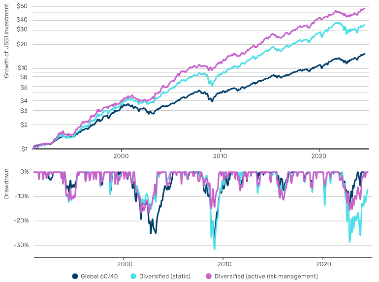
Source: Man Group. January 1991 to July 2024. Time period selected based on availability of reliable data. Simulated past performance is not indicative of future results.
Table 1. Performance and risk statistics of global investment strategies
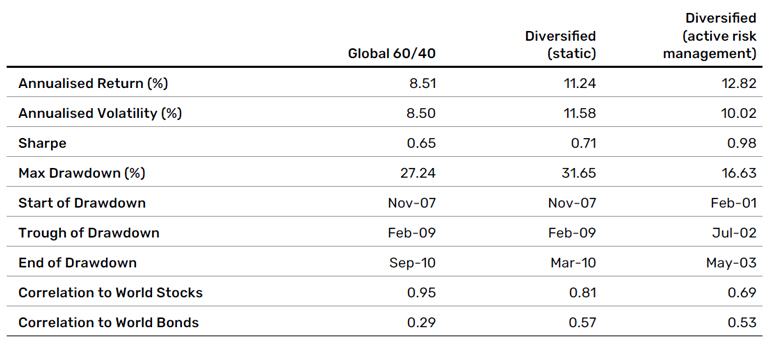
Source: Man Group. January 1991 to July 2024. The performance data is simulated and is shown for information purposes only. The simulated data does not represent actual performance of the strategy or of a fund and it should not be used as a guide to the future. This approach has inherent limitations, including that results may not reflect the impact material economic and market factors might have had on the investment manager’s decision-making and/or the application of any trading models had the strategy or fund been managed throughout the period over which the simulated performance is illustrated.
Staying active to stay healthy
There is a large amount of randomness in financial markets, particularly in relation to the direction of prices moves. However, some other features of market prices are more predictable, namely those relating to risk and diversification. Given our experience managing systematic hedge funds since the 1980s, we believe that it is possible to use this predictability to our advantage; to improve risk-adjusted returns without the need to forecast the direction of returns.
In general, strategic allocations do not adjust for changes in the riskiness of assets but assume that different assets have different long-term volatility levels and that little can or should be done about shorter-term fluctuations in riskiness. While historical returns have been poor forecasts of future returns, historical volatility has been a good forecast of future volatility. Equity volatility can vary wildly through time, lending importance to accurate forecasting. Indeed, some of the periods of highest equity market volatility have coincided with periods of negative returns (the leverage effect).
In this context, we advocate using active risk management to improve risk-adjusted returns and to mitigate tail risks. Employing risk targeting to control short- and medium-term risk by adjusting investment exposures can restrict a portfolio’s volatility from rising too high (which is associated with an increased risk of drawdown), or too low (which is associated with a risk of undershooting growth targets). Risk targeting can also be used to allocate risk consistently between asset classes, improving diversification.
In short, we believe there are four key ingredients for actively navigating turbulent markets:
1. Balance risk across asset classes to provide robustness to the macroeconomic environment
2. Improve risk-adjusted returns through short-term risk forecasting rather than return forecasting
3. When conditions are favourable, take enough overall risk to achieve return targets
4. Manage the tails
1. A rigorous mathematical treatment of this can be found in (Hoyle & Shephard, 2018).
Bibliography
Harvey, C. R., Hoyle, E., Korgaonkar, R., Rattray, S., Sargaison, M., & Van Hemert, O. (2018). The Impact of Volatility Targeting. The Journal of Portfolio Management, 45(1), 14-33. doi:10.3905/jpm.2018.45.1.014
Hoyle, E. (2020). The Glidepath Confusion. Man AHL working paper. doi:10.2139/ ssrn.4750204
Hoyle, E., & Shephard, N. (2018). Volatility Scaling’s Impact on the Sharpe Ratio. Man AHL and Harvard University working paper. doi:10.2139/ssrn.3279787
Neville, H., Draaisma, T., & Funnell, B. (2022). Varying by Degress: Fire & Ice 2.0. Man Institute. Retrieved from https://www.man.com/maninstitute/varying-by-degrees-fire-and-ice
Neville, H., Draaisma, T., Funnell, B., Harvey, C. R., & Van Hemert, O. (2021). The Best Strategies for Inflationary Times. The Journal of Portfolio Management, 47(8), 8-37. doi:10.3905/jpm.2021.1.274
Tobin, J. (1958). Liquidity Preference as Behavior Towards Risk. Review of Economic Studies, 25(2), 65-86. doi:10.2307/2296205
You are now leaving Man Group’s website
You are leaving Man Group’s website and entering a third-party website that is not controlled, maintained, or monitored by Man Group. Man Group is not responsible for the content or availability of the third-party website. By leaving Man Group’s website, you will be subject to the third-party website’s terms, policies and/or notices, including those related to privacy and security, as applicable.