The Road Ahead: How To Leave Your Child A Million Dollars

Before we start a disclaimer. You can put us in the camp that says a financial inheritance generally takes more than it gives to the beneficiary. Few things more impressive than a self-made man. So be careful taking that opportunity away from them, is our parenting tuppence worth.

Still, anything for a snappy title. And indeed it gives us the opportunity to demonstrate a) the power of combining assets and strategies that diversify, b) the optimal ways of making said combinations but also c) the limits thereof. As multi-asset investors this is our daily bailiwick, albeit on an institutional rather than individual level. For the majority of people who do not share our nerdy interest in portfolio construction, there will hopefully be some interesting statistics and bon mots along the way.

To start, some assumptions. The average starting salary for a university graduate in the United States is USD55,000.¹ The Bureau of Labor Statistics puts the long term growth rate of average hourly earnings at 3%. If we take this and assume a 40-year working life, that would mean we can take a heuristic that a typical worker today will end their career on USD179,000. Further assume that our theoretical worker dies at 79 (the current average age of death in the US), invests monthly while working, and that his savings pool continues to compound at the rate of return achieved during his working life until retirement. To keep things simple let’s say the current all-in personal tax rate of 28% stays static.² What level of saving rate and return above inflation will achieve an inheritance for his child of USD1 million in today’s money? Please show your working…

Fret not. We’ve done the maths for you, answers in Figure 1. Over the last 70 years the US saving rate has averaged 9%. Let’s assume five percentage points of this are required to provide a nest egg for retirement income, meaning we have an effective saving rate of 4%. At this level we would require a return ahead of inflation of 8.3% to generate 1 million 2022 dollars by the date of death.

Figure 1. Size of Inflation-Adjusted Legacy at Death

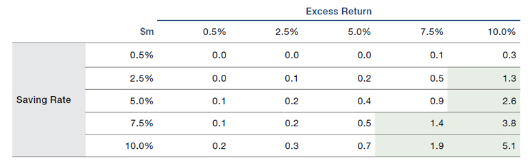
Source: Bloomberg, Shiller, Man Solutions; as of 31 October 2022.

The obvious next question is what rate of inflation do we expect our hypothetical worker to feel. Figure 2 shows the average annual price rises experienced by a person who had a 40-year career, a 15-year retirement, then shuffled off the perch. There is a surprising amount of variability. Someone dying in the 1920s and 1930s would have experienced only 1% inflation per annum through their adult lives. Someone dying in the mid-1990s would have felt 4.5%, which has moderated to around 4% for someone dying today. If we take the average across the whole chart, we get 3%. Which seems as sensible a number as any.

Figure 2. Average Rate of Inflation Felt During Adult Life for an Individual Dying in a Given Year

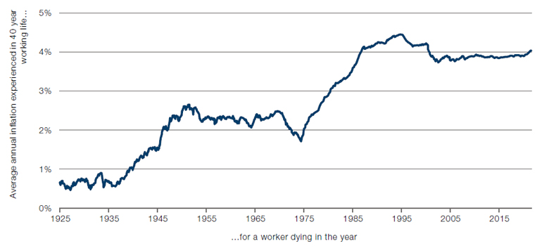
Source: Bloomberg, Shiller, Man Solutions; as of 31 October 2022.

So the bottom line is that we need a nominal return of 11.3%. Which feels punchy. But is it insurmountable? In Figure 3 we give various summary statistics for the three main asset classes as we see them – equities, bonds and alternatives – over the past 100 years. Here are four observations:

1. There is no unlevered combination of assets which will realise our desired 11% return. A 100% equity portfolio only gets us 10%, and with 60%+ max drawdown, which is likely to be unacceptable to most investors;
2. The average pairwise correlation between the three assets is 0.1, they therefore represent attractive diversifying components of a portfolio;
3. Equities have the advantage of producing the best return per unit of leverage, but the disadvantage of a drawdown which is likely too painful for many investors, and a distribution which is heavily leptokurtic, indicating an increased preponderance to tail events;
4. While alternatives are the most attractive asset in Sharpe ratio terms, and almost perfectly normally distributed, that must be weighed against a higher correlation with equities (although still low in the absolute sense), as well as, from a practical perspective, a higher fee load (which we do not consider here for convenience reasons).

Figure 3. Summary Statistics (Above) and Correlation Matrix (Below) for Equities, Bonds and Alternatives Over the Last 100 years³

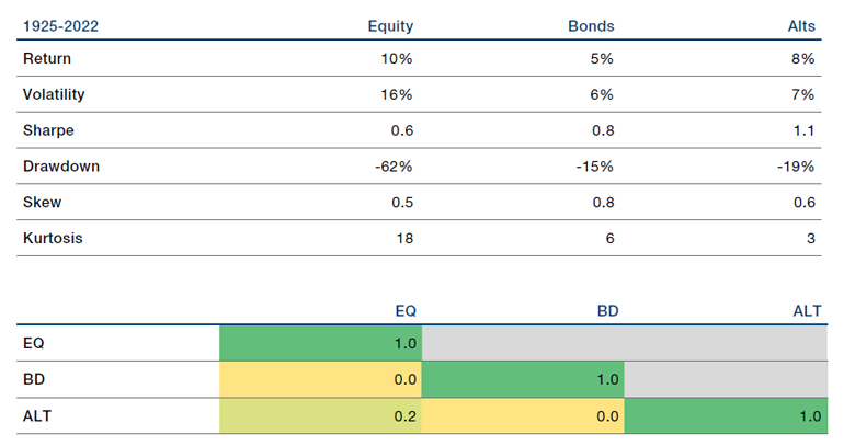
Source: Bloomberg, Shiller, Man Solutions; as of 31 October 2022.

How best to combine these assets? The temptation is strong to torture the data into a max Sharpe confession, but that wouldn’t be fair. Instead, we cue off volatility as the most predictable statistic. To see this observe Figure 4, where we show 10-year trailing annualised return and volatility for US equities. Volatility has three long periods of relative stability: 1810-1833 (where it stays around 5%), 1873-1929 (12%) and 1950 to present (15%). Return on the other hand moves in much more directional patterns.

Figure 4. Ten-Year Rolling Volatility and Return for US Equities

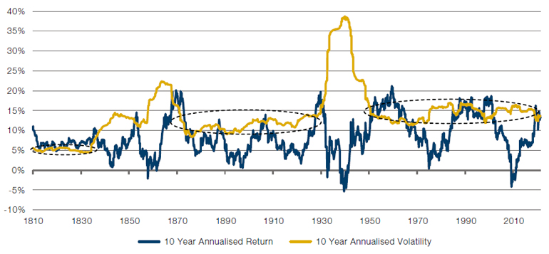
Source: Bloomberg, Shiller, Man Solutions; as of 22 November 2022.

Rounded to the nearest ten, the allocation that gets closest to equalising the risk contribution from each of the three assets is 20% equity, 40% bonds, 40% alternatives. However, this only gets us a 7.5% return. To get to our 11.3% number we must lever this portfolio 1.5x to reach 30/60/60. In Figure 5 we show the performance of both these portfolios with summary statistics for 30/60/60.

Figure 5. Long Term Performance 20/40/40 and 30/60/60 Portfolios

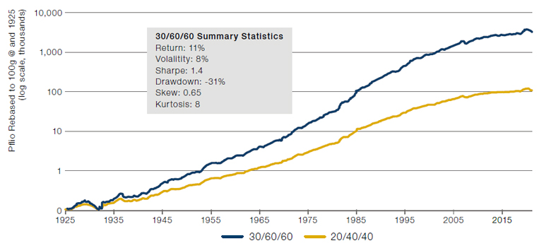
Source: Bloomberg, Shiller, Man Solutions; as of 22 November 2022.

What can we say about the resulting portfolio:

1. Despite being 1.5x levered it has just two-thirds of the volatility of a 100% equity portfolio. Leverage is a dirty word and, in the wrong hands, rightly so. But thought of in volatility terms it is perhaps more accurate to think of it as ‘exposure management’;
2. A similar effect is seen if one defines risk according to drawdown rather than overall volatility, with the resulting portfolio delivering half the max drawdown of a non-levered equity-only vehicle;
3. The diversification inherent in the low correlations between the three assets shows up in increased risk efficiency. The 1.4 Sharpe is higher than for any of the assets individually (per Figure 3);
4. The distribution of returns is not far off normal (taking the heuristics that -1 to +1 is normal skew and -7 to +7 is normal kurtosis). This means that if the 100 years of data we show in Figure 5 are any guide, our investor can expect a 10% or more YoY drawdown less than 3% of the time, and a 5% or more MoM drawdown about 1% of the time.

Now clearly, we plucked the USD1 million present value dollars hurdle out of thin air. But whatever your financial goals, either as an individual or an institution, we think this way of thinking is a useful starting point. But for the individual we repeat the warning we began with – large financial inheritances often weigh heavy, like the dead Albatross around the neck of the Ancient Mariner.

1. Based on October 2022 data from Zippia.
2. As estimated by the OECD
3. Equity is Professor Shiller’s US equity series. Bond is represented by the UST10 and is taken from GFD. Alternatives represent a portfolio of equal capital weights to commodities, trend and equity long/short. Commodities are proxied with an equal weight portfolio of all futures contracts as they appear through history. Pre-1946 this is based off work done by AQR and post that date we use futures contracts from the Man AHL database. Trend is a long-term portfolio constructed by Many AHL which aims to replicate the exposures of the BTOP50 index at 15% volatility, covering commodities, FX, equities and bonds. Equity long/short is volatility scaled equal weight portfolio across the Fama-French SMB, HML and Mom. factors, as well as the AQR BAB and QMJ factors. All returns are nominal and annualised.