Introduction
With the rise of systematic trading and machine learning-driven investment, investors are moving towards faster, higher turnover strategies. For those strategies, the measurement of costs is crucial.
The easiest way to boost the alpha of a trading strategy is to reduce costs. With the rise of systematic trading and machine learning-driven investment, investors are moving towards faster, higher turnover strategies. For those strategies, the measurement of costs is crucial and can potentially render some strategies unprofitable if not properly considered.
Common approaches of measuring such impact generally only focus on a single transaction, or parent order, at a time. However, in many cases, those orders are correlated and the impact of the first order will affect the execution of future orders. In this article, we investigate the case where parent orders, also called metaorders, themselves are correlated. Here we review a new technique called the expected future flow shortfall, or EFFS for short, which we propose in a research paper (see reference at the bottom).
Metaorders, Child Orders and Slippage
Consider portfolio managers making investment decisions and expressing these decisions in the form of desired trades, i.e., in shares to buy or sell.
If the desired trade is small – e.g., if it is equal to 100 shares – the whole size is going to be submitted to the exchange in a single order. However, in many cases, submitting the whole quantity may be impractical (for example, the desired trade size may exceed the total liquidity available at the exchange at that moment in time). In this case, the desired trade is typically split by the execution agent into smaller suborders and executed incrementally. Those suborders are called child orders. We will call the desired trade that was communicated to the execution agent a metaorder.
When the investment decision is made, the latest available market price (such as the latest mid-point price, or previous closing auction price) is noted. This is known as the decision price. When the instruction arrives at the execution agent, the latest available market price is noted and is called the arrival price. We assume that the processes of communication are very fast and efficient, so that the decision and arrival prices coincide, and accordingly these terms are used interchangeably in what follows. Given that the market moves while the child orders are executed, those are in general filled at different prices than the decision price. The difference between the decision price and the volume weighted trade prices of the child orders is known as slippage. Slippage is a common metric to measure execution cost due to price impact.
Looking at a single metaorder, it is hard to perceive the impact of our trading, as market moves are generally two orders of magnitude larger. We illustrate this in Panel A of Figure 1 which shows the evolution of 1,000 simulated price moves during the ‘continuous’ execution of a buy metaorder starting at a decision price of 100. At first glance, it seems that roughly half of the prices go up and half go down, which is due to general market moves unrelated to our trading. However, looking more closely, for buy orders, the price path moves higher in slightly more than 50% of cases, while moving lower in the remainder.
On average, across many metaorders, the execution price path is slightly higher than the decision price. This is not immediately clear in Panel A because the mean impact curve looks flat, but this is simply due to the plotting scale given that impact is much smaller than typical price moves. In Panel B of Figure 1, we focus on a narrower range of prices to see how the impact drives prices higher. Comparing the two panels, it is obvious that the standard deviation of the price moves in Panel A (approximately 100 basis points) is much larger than the impact (approximately 10 basis points).
Figure 1. Market Impact Based on 1,000 Monte Carlo Simulations
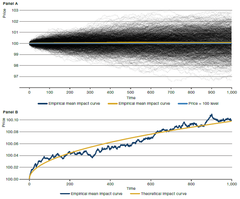
Source: Man Group. For illustrative purposes.
Note: Panel A shows 1,000 simulated mid-price moves (black) during the execution of a buy metaorder. The average of those mid-price paths gives the empirical mean price impact curve that is shown in green, together with the theoretical curve in red. These empirical and theoretical impact curves only are much clearer in Panel B that focuses on a narrower range of prices. Note that price impact is around one to two orders of magnitude smaller than typical mid-point price moves, as becomes apparent when comparing Panels A and B.
Hypothetical results are calculated in hindsight with modelling assumptions. Since trades have not actually been executed, hypothetical results may have under- or over-compensated for the influence, if any, of certain market factors. Later, we apply our method to actual trading data.
Persistent Market Impact and Its Effect on Subsequent Metaorders
The broad stylised facts of market impact are as follows: the mid-price is, on average, increasing throughout the buy metaorder duration and is likely to start reverting after the metaorder finishes trading. It may or may not revert completely. The part of the impact that never reverts (or is extremely slow to revert) is called permanent impact. An illustration of the price impact of an isolated buy metaorder is presented in Figure 2. The price trajectory over the metaorder can be linear or non-linear (typically concave).
Figure 2. Stylised Representation of Average Permanent Versus Temporary Price Impact
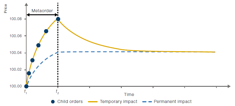
Source: Man Group. For illustrative purposes.
The exhibit shows the average effect of the execution of a metaorder consisting of six (child) orders, as well as the resulting average temporary and permanent price impact. The decision price (shown here as 100) is the price that would be expected at each time point if there was no trading.
Direct measurement of the permanent market impact is practically impossible, as subsequent metaorders may start trading before the reversion of the initial metaorder has finished. For large-scale asset managers, it is often impractical to submit the whole desired amount in one metaorder. Indeed, the amount may not even be possible to trade over a full day. This leads to an autocorrelation effect: buy metaorders tend to be followed, on average, by buy metaorders, and vice-versa for sell metaorders. Figure 3 presents a stylised picture for trading two consecutive buy metaorders.
Figure 3. Execution of Two Metaorders With ‘Relaxation’ Time In Between
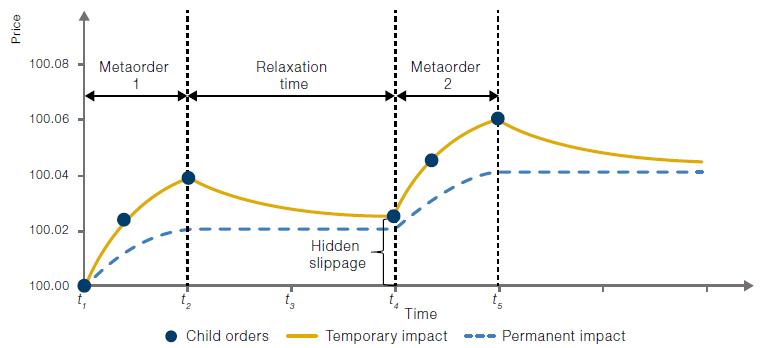
Source: Man Group. For illustrative purposes.
The ‘relaxation’ time, between t2 and t4, allows part of the temporary impact of the first metaorder to decay. However, the decision price of the second metaorder is still affected by the impact of the first metaorder, leading to hidden slippage.
Direct measurement of the permanent market impact is practically impossible, as subsequent metaorders may start trading before the reversion of the initial metaorder has finished.
Figure 3 illustrates that the decision price of the second metaorder is approximately 100.025 – elevated above 100 by the impact of the first metaorder (both temporary and permanent).
There are several insights here. First, the difference in price at time t4 (100.025 to 100) is not reflected in the usual slippage metric for either metaorder. We sometimes refer to the price of 100 as the cleaned price and 100.025 as the dirty price impacted by our trading. Second, if the profitability of the trade idea depends on the execution of both metaorders, it is essential to consider the impact of the first metaorder on the price used to benchmark the second metaorder. Such considerations may also influence the sizing decision of each metaorder for best overall execution.
Research or paper trading often assumes that both metaorders could be executed at a price of 100 plus implementation shortfall. This would misrepresent the viability of the trade idea. This effect on the price, cost and profitability of the subsequent trades is sometimes called hidden slippage, as it is not reflected in the traditional slippage metric. Our proposed expected future flow shortfall (‘EFFS’) model enables measurement of this hidden slippage.
The Expected Future Flow Shortfall Model
In setting up the EFFS model, there are a few things to note. First, we assume that metaorders are broken down in child orders of the same side, i.e., if the metaorder is a buy order, all the child orders will be buy orders as well. Second, rather than just focusing on the cost of the current trade, we are interested in the effect of the price move on any future metaorders (this is estimated using the expected future flow or EFF of metaorders). The impact a price move has on the EFF is what we call the expected future flow shortfall or EFFS. In other words, the EFFS of a given trading period is equal to the immediate price move from the given to the next period multiplied by the EFF following this period. The EFF needs to be estimated from data. Intuitively, for correlated order flow, a buy order is more likely to be followed by buy orders so that the net effect on the EFF is positive. Moreover, we expect this effect to be more pronounced for a larger buy order. Quantitatively, the strength of this effect can be estimated from the data. This is explained in more detail in the research paper cited at the end of this article.
Despite the conceptual simplicity of the propagator model, there are several hurdles to overcome in order to implement it in practice. The main one is that it typically requires a long history of trading data.
Another approach to deal with the market impact of correlated order flow is the so-called propagator model. This model makes the simplifying assumption that each metaorder can be treated separately, and that the effect of each metaorder can be summed linearly. Using this, the market impact of each realised trade can be subtracted from the observed prices to obtain cleaned prices, i.e., the prices that would have been observed without the impact of the trading. These hypothetical prices can be used to calculate the cleaned P&L of the strategy. The difference between this cleaned P&L and the realised P&L provides a measure of the additional effect on P&L beyond standard slippage, similar in spirit to the impact data captured by the EFFS.
Despite the conceptual simplicity of the propagator model, there are several hurdles to overcome in order to implement it in practice. The main one is that it typically requires a long history of trading data, with potentially millions of metaorders needed for adequate estimation. This provides the propagator model limited adaptivity, thus making it ill-suited to identifying changes in execution quality over shorter periods of time.
To illustrate the strengths of our EFFS method and relative performance when compared to a propagator model approach, we applied both methods to metaorders from a proprietary trading strategy. We report estimates for every month between January 2018 and January 2019 in Figure 4. To focus on relative performance, we normalise the measurements so that the propagator estimate equals 100% every month. To be clear, a value of 80% means that the EFFS has 80% of the propagator shortfall.
Figure 4. EFFS Versus Propagator Monthly Estimates
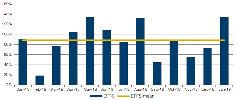
Source: Man Group. Between January 2018 and January 2019.
Note: We show the monthly average shortfall computed using the propagator model and the EFFS model. Statistics are based on approximately 730,000 trades. The propagator model is normalised to 100%. Hence, a value of 80% means that the EFFS model returns a shortfall that is 80% of the size of the propagator model. The EFFS model gives estimates that are close to estimates from the propagator model when averaged over the entire year. Note the larger difference in the volatile month of February 2018.
There are two important takeaways from Figure 4:
- Over the entire sample period, the simple EFFS model performs similarly to the difficult-to-estimate propagator model. The average difference in dollar terms between the two models over the period is approximately 12% and only 6% if the tumultuous month of February 2018 is excluded;
- The performance of the EFFS in this month points to the second important observation: the EFFS estimate is much more adaptive as it uses only one month of data. The propagator model, in contrast, uses approximately one year of data, so is naturally smoother and much less sensitive to changes in the distribution of price moves and trades.
Conclusion
Our method is intuitive and straightforward to implement – we provide simulation evidence in a number of different market scenarios, illustrating that the EFFS approach has distinct advantages over alternative approaches.
The adaptability of the EFFS method is also illustrated by computing the median of the absolute change in shortfall month-on-month, which is 47% for the EFFS model and only 15% for the propagator model. The relatively high variance in the EFFS estimates is exactly what we would expect given the estimates rely on standard execution slippage measurements calculated per metaorder which, as already noted, are extremely variable, being strongly affected by price moves during the metaorder.
In this era of machine learning and big data, trading occurs much more frequently. As such, it is increasingly important to be as efficient as possible in executing trades. Common approaches suffer from a type of myopia: impact is only measured for the current transaction. However, in many cases, orders are correlated and the impact of the first order will affect the execution of future orders. Here we review a new technique which we call the EFFS – the expected future flow shortfall – to address this issue.
Our method is intuitive and straightforward to implement – we provide simulation evidence in a number of different market scenarios, illustrating that the EFFS approach has distinct advantages over alternative approaches. We also provide a real trading example using proprietary data. Our empirical analysis reveals that the EFFS performs competitively with more complex and data-hungry approaches, such as the propagator model, and is much more reactive to changing market conditions.
In summary, the theoretical properties and empirical results point to the benefits of deploying the EFFS formula as a simple way to estimate the trading effects on P&L beyond standard slippage estimates. This is particularly important for faster strategies and those with autocorrelated order flow.
To read the full academic research, click here.
Hypothetical Results
Hypothetical Results are calculated in hindsight, invariably show positive rates of return, and are subject to various modelling assumptions, statistical variances and interpretational differences. No representation is made as to the reasonableness or accuracy of the calculations or assumptions made or that all assumptions used in achieving the results have been utilized equally or appropriately, or that other assumptions should not have been used or would have been more accurate or representative. Changes in the assumptions would have a material impact on the Hypothetical Results and other statistical information based on the Hypothetical Results.
The Hypothetical Results have other inherent limitations, some of which are described below. They do not involve financial risk or reflect actual trading by an Investment Product, and therefore do not reflect the impact that economic and market factors, including concentration, lack of liquidity or market disruptions, regulatory (including tax) and other conditions then in existence may have on investment decisions for an Investment Product. In addition, the ability to withstand losses or to adhere to a particular trading program in spite of trading losses are material points which can also adversely affect actual trading results. Since trades have not actually been executed, Hypothetical Results may have under or over compensated for the impact, if any, of certain market factors. There are frequently sharp differences between the Hypothetical Results and the actual results of an Investment Product. No assurance can be given that market, economic or other factors may not cause the Investment Manager to make modifications to the strategies over time. There also may be a material difference between the amount of an Investment Product’s assets at any time and the amount of the assets assumed in the Hypothetical Results, which difference may have an impact on the management of an Investment Product. Hypothetical Results should not be relied on, and the results presented in no way reflect skill of the investment manager. A decision to invest in an Investment Product should not be based on the Hypothetical Results.
No representation is made that an Investment Product’s performance would have been the same as the Hypothetical Results had an Investment Product been in existence during such time or that such investment strategy will be maintained substantially the same in the future; the Investment Manager may choose to implement changes to the strategies, make different investments or have an Investment Product invest in other investments not reflected in the Hypothetical Results or vice versa. To the extent there are any material differences between the Investment Manager’s management of an Investment Product and the investment strategy as reflected in the Hypothetical Results, the Hypothetical Results will no longer be as representative, and their illustration value will decrease substantially. No representation is made that an Investment Product will or is likely to achieve its objectives or results comparable to those shown, including the Hypothetical Results, or will make any profit or will be able to avoid incurring substantial losses. Past performance is not indicative of future results and simulated results in no way reflect upon the manager’s skill or ability.
You are now leaving Man Group’s website
You are leaving Man Group’s website and entering a third-party website that is not controlled, maintained, or monitored by Man Group. Man Group is not responsible for the content or availability of the third-party website. By leaving Man Group’s website, you will be subject to the third-party website’s terms, policies and/or notices, including those related to privacy and security, as applicable.