Introduction
Trading moves prices. This statement has been an immutable law of financial markets since time immemorial. All trades generate price impact – with buys pushing prices up, sells pushing prices down, and later trades experiencing impact from those that have gone before.
Previous studies have considered optimal execution of individual trades. In contrast, our focus is minimising price impact over a pair of trades. The results reported here are the first steps in a new research direction, with the ultimate goal of optimising transaction costs over sequences of multiple trades.
Previous Research: The STSH Case
Previous research on optimising transaction costs focuses on executing a single trade over a single time horizon – the ‘STSH’ case discussed in the full academic paper. The smallest STSH transaction cost is achieved by splitting the single parent order into a sequence of child orders comprising:
- A pair of block trades executed instantaneously at the beginning and end of the available execution time horizon; plus
- Continuous trading executed throughout the execution period, potentially with a time-varying intensity.
Our research embarks on minimising the combined market impact (transaction cost) of a pair of trades executed one after the other.
Figure 1 illustrates these components. The block trade at the start of the execution period arises because the STSH setup assumes no market impact has accumulated at that point, so trading with high intensity at t=0 incurs only a small cost. In contrast, the block trade at the end of the execution period arises because the STSH setup assumes all impact beyond t=T1 (when trading finishes) can be ignored. Neither of these assumptions is valid when sequences of trades are the focus, since impact at the start of any execution interval depends on what has gone before, and impact generated at the end of each interval matters for the next trade. In practice, most market participants deal with this by heavily discounting such block trades in their execution schedules. For example, the widely used Time Weighted Average Price (‘TWAP’) and Volume Weighted Average Price (‘VWAP’) trajectories target only continuous schedules.
Our research embarks on addressing this by minimising the combined market impact (transaction cost) of a pair of trades executed one after the other.
Figure 1. The Components of an Optimal STSH Trajectory
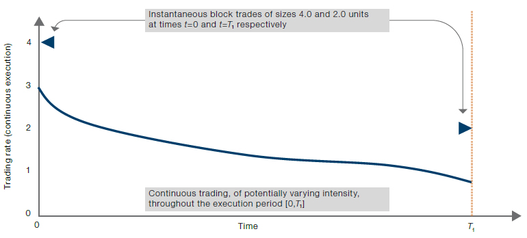
Source: Man Group. For illustrative purposes only.
Note: In the special case where the trading impact is linear and has exponential decay, then the continuous trading component of the optimal STSH trajectory occurs at constant rate over the full execution period [0,T1].
Details of Our Research
The price impact of a trade can be decomposed into two components: instantaneous price impact, which is the immediate shock to market prices; and a decay component, representing the gradual dissipation of the instantaneous price shock over time. Instantaneous price impact is higher for larger orders, and for simplicity we assume it is a linear function of order size. Likewise, we assume an exponentially decreasing decay component.
We consider two trades, with the first to be completed before the second commences. For simplicity, and without loss of generality, we assume the first trade is a buy of V[0,1]>0 shares that is to be executed over period [0,T1], where the end-time of the execution horizon (T1) is known. Exactly as for the STSH case, the market impact of the first trade is the difference between the total purchase price of the V[0,1] shares and the price at which they could theoretically have been purchased when trading commenced at time t=0. This first trade is said to be benchmarked using price S0, where S0 denotes the market price at time t=0.
We assume the second trade is of size V[1,2] and is to be executed over the period [T1,T2], with a positive or negative V[1,2] value corresponding to a buy or sell respectively. We assume the end of the second execution interval (T2) is known, consistent with our setup for the first trade.
We explore two ways of benchmarking the second trade:
- Separate costs: Here we benchmark the second trade using ST1 which denotes the market price at time T1. This is the standard approach among practitioners for monitoring transaction costs. We refer to this two-trades separate costs approach as TTSC;
- Hybrid costs: We decompose the second trade V[1,2] into the sum of its predicted value, V[1,2],p say, and an amend part V[1,2],a that becomes known only at time T1. The predicted part V[1,2],p is benchmarked using S0 while the amend part V[1,2],a is benchmarked using ST1. We refer to this two-trades hybrid costs approach as TTHC.
The TTHC problem accommodates the case where both the size and direction (buy or sell) of the second trade are uncertain in advance. This most closely resembles the practical situation faced by systematic investment managers like Man AHL.
Our Findings
First, as a straw-man baseline, we find that adopting the optimal STSH solution independently over the two orders (we term this the myopic strategy) can significantly underperform compared to optimising a shortfall cost that accounts for both periods. Figure 2 illustrates such a situation for a buy trade of size 1.0 units (of say 1,000 shares) followed by a second buy of size 3.0 units. Here the myopic strategy underperforms the optimal TTSC and TTHC solutions by 14% and 11% under the respective two-period impact formulations.
Adopting the optimal STSH solution independently over the two orders can significantly underperform compared to optimising a shortfall cost that accounts for both periods.
Second, issues can arise even when we account for both execution periods. For example, the optimal TTSC solution may exhibit significant backloading, as shown in the middle panel of Figure 2. Here the first buy trade is maximally backloaded, delivering its entire size to market as an instantaneous block trade just before the second trade begins. Such extreme backloading can arise in optimal TTSC solutions because the second trade is benchmarked using price ST1 , a quantity that is not exogenous to the system undergoing optimisation but incorporates the impact of the first trade. This makes the overall TTSC problem gameable. In this example, optimising the TTSC impact exploits this weakness by scheduling the first trade to maximally drive-up the second benchmark price (ST 1) so that the downwards price decay which follows may benefit the purchase price for the second trade. In contrast, even though the TTHC impact uses ST1 to benchmark the amend part of the second trade, extreme gaming like this does not arise in the optimal TTHC solution because the amend trade is equiprobably a buy or sell. In fact, optimal TTHC execution schedules typically frontload their trajectories compared to optimal TTSC solutions, as seen in the right panel in Figure 2.
Figure 2. Execution Schedules
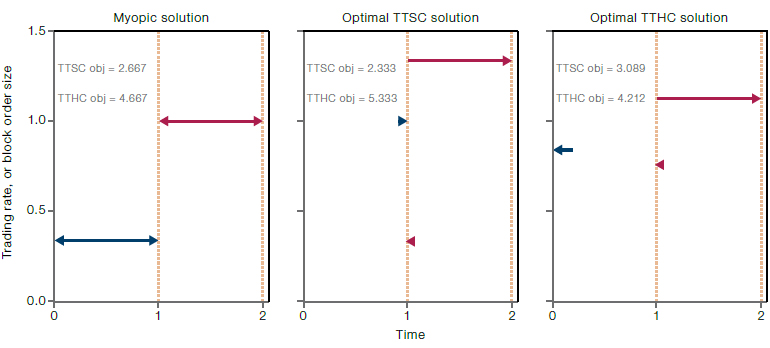
Source: Man Group. For illustrative purposes only.
Note: Execution schedules obtained for (T1,T2)=(1,2) in the case of two buys, with V[0,1]=1 and V[1,2]=3. The triangular symbols denote instantaneous block trades while the horizontal lines depict continuous trading at constant rate. The left-hand panel shows the myopic execution schedule obtained by applying the optimal STSH solution independently to both trades. The middle panel shows the optimal TTSC solution and the right-hand panel shows the optimal TTHC solution (obtained by setting V[1,2],a≡0). Compared to the optimal TTSC and TTHC solutions, the myopic solution underperforms by approximately 14% (2.667/2.333) and 11% (4.667/4.212) respectively under the corresponding TTSC and TTHC impact formulations. In the middle panel, the TTSC impact reports less than 50% of the cost of the optimal TTSC solution when the true cost is given by the TTHC metric (2.333 versus 5.333).
Table 1. Details of the Various Solutions
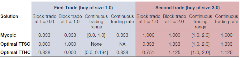
Source: Man Group. For illustrative purposes only.
Note: In contrast to the myopic solution where the first and second continuous trading periods cover the full range of their respective execution horizons, optimal TTSC and TTHC solutions may exhibit trading gaps within their schedules, like those shown here. The volume traded within each period of continuous trading is given by the product of the corresponding trading rate and the duration of the continuous trading range. For example, for the optimal TTHC solution the first period of continuous trading involves purchasing 0.838×(0.194-0.0)≈0.163 units, while the second corresponds to a purchase of 1.125×(2.0-1.0)=1.125 units.
The widely used TTSC impact metric may significantly understate the cost of optimal TTSC solutions when the true cost is given by the TTHC metric.
Third, we find that the widely used TTSC impact metric may significantly understate the cost of optimal TTSC solutions when the true cost is given by the TTHC metric. This has potentially wide consequences for asset managers, as they run the risk of significantly understating the true cost of their trading if they use separate costs, e.g. for simplicity or convenience, when their real objective is hybrid costs. This is problematic even if explicit order optimisation is not used, as ad hoc experiments with backloading that happen to benefit the separate costs criterion may lead to apparent improvements in execution while actually making things worse.
Additional buy-buy and buy-sell examples that contrast the myopic, TTSC and TTHC optimal execution schedules are provided in the academic paper, covering both the deterministic case (as in Figure 2) and the stochastic case where neither the size nor direction of the second trade is known in advance. We also provide examples where any periods of continuous trading are forced to span their respective execution horizons and observe that this induces only negligible increases in total cost. Further practically important extensions of the two trade case are possible but are yet to be studied, e.g. when inventory from the second trade may be migrated for execution into the first period. Such a scheme requires discretion to be given to execution systems in anticipation of unconfirmed future orders. However, such flexibility is not standard practice within the industry. We do not discuss this further, but note it is another important execution problem that falls outside the scope of standard STSH solutions.
Conclusion
Reducing transaction costs is an important goal for any institution that trades in financial markets. As such, optimising trade execution strategies is a well-studied problem with a wide literature.
This study provides a stepping-stone towards the general case of multiple trades and execution horizons.
Our full academic paper first presents a novel and general solution method for the case of a single trade that is executed as a sequence of sub-trades. We then analyse the case of two sequential orders, including the case where the size and direction of the second are uncertain at the time the first is initiated. We obtain the optimal execution strategy under two different cost functions. First, we minimise the total cost when each order is benchmarked to the price at its initiation, the total separate costs approach widely used by practitioners. Although simple, we show that optimising total separate costs can significantly understate the real costs of trading and lead to detrimental backloading.
We overcome these issues by introducing a new cost function that splits the second order into two parts, one that is predictable in advance and a residual that is not.
To the best of our knowledge, this study is the first to consider optimal execution within such a framework and provides a stepping-stone towards the general case of multiple trades and execution horizons.
To read the full academic paper, click here.
You are now leaving Man Group’s website
You are leaving Man Group’s website and entering a third-party website that is not controlled, maintained, or monitored by Man Group. Man Group is not responsible for the content or availability of the third-party website. By leaving Man Group’s website, you will be subject to the third-party website’s terms, policies and/or notices, including those related to privacy and security, as applicable.