Skewness

Skewness is often thought of as a simple measure of asymmetry in the distribution of market returns. The board investigated more thoroughly the concept of skewness and how it applies to both markets and investors.

OVERVIEW

• Skewness is an imperfect measure of asymmetry in return distributions. It is sensitive to outliers, and requires very large quantities of data to accurately estimate. There are better, statistically more robust, estimators of asymmetry available.
• Economic theory can help us better estimate skew. Due to the difficulties in empirically measuring skew, we can supplement the information from our observations with economic theory. For example, IPOs are predisposed to be positively skewed due to the winnertake-all economics of the underlying industry.
• Investors display a preference for positively skewed return profiles. This preference for skew can be modelled by behavioural economics using Prospect Theory, and may have evolutionary roots.
• Volatility scaling is helpful in managing skew. In equity markets, we often see falls in prices lead to an increase in volatility – the statistical leverage effect. This can cause negative skewness in returns. However, if you scale your positions with respect to volatility, then you can potentially remove or even reverse the skewness of the unconditional returns.
• Dynamic Trading allows one to transform the asymmetry in asset returns. CTAs provide an example of this transformation. They produce a positively skewed return profile by trading univariate momentum.
• Managing skewness in a portfolio is important. It can be accomplished by diversifying the signal set whilst being mindful of leverage. Allocating to strategies with positive skew, such a momentum, helps. One should always be very careful about relying alone upon historical estimates for skew, and should incorporate theory into ex-ante skew estimates.

INTRODUCTION

The board, whose members bring diverse perspectives and deep expertise, consists of:

• Nick Barberis - Professor of Finance at the Yale School of Management – one of the world’s leading experts in behavioural finance.
• Campbell Harvey - Professor of Finance at the Fuqua School of Business at Duke University and Editor of the Journal of Finance from 2006-2012 – a leading financial economist with a focus on the dynamics and pricing of risk.
• Neil Shephard - Professor of Economics and of Statistics at Harvard University. He was the founding director of the Oxford-Man Institute of Quantitative Finance in Oxford and directed it from 2007-2011 – one of the top theoretical and applied econometricians.

These distinguished academics were joined by Matthew Sargaison, Chief Investment Officer of Man AHL, Nick Granger, former Portfolio Manager of Dimension, Co-head of Research and Deputy Chief Investment Officer of Man AHL, Anthony Ledford, Chief Scientist of Man AHL, Greg Bond, Head of Research of Man Numeric, and Paul-James White, Quantitative Analyst at Man AHL.

Before launching straight into the discussion, we point the interested reader to the appendix for a very brief survey about skewness.

 

THE DISCUSSION

1. What is skewness? What are the different ways of measuring it?

Neil Shepherd (NS): Skewness is defined to be the third moment of a distribution. Mathematically it is straightforward. It has the downside that it is challenging to estimate. In order to estimate the third moment with a reasonable amount of data, one needs a central limit theorem, which itself requires the sixth moment to exist. In financial data, which tends to be fat tailed, this is rarely the case. The result is that our estimate for skew is very sensitive to outliers. The problem is even more severe if one believes skew is time-varying. Often there simply isn’t enough data to obtain a meaningful estimate.

Anthony Ledford (AL): It is important to pin down exactly how much data one requires for an accurate estimate of skew. For example, is a value of 0.3 meaningfully larger than 0.29? Probably not, at least on financial data reported daily without an enormous history.

Matthew Sargaison (MS): There is also the issue of the return period used. Measuring the skew of a strategy using daily returns can give a very different result to using monthly returns. Due to the difficulties in estimation in practice, skew is almost a state classifier: negative, positive or zero. The specific value matters much less.

AL: People often use the word skew to refer to the asymmetry of a distribution or even tail risk. Often they are worried about whether the probability of a large negative return is greater than the probability of a large positive return. These are different properties and should be studied separately.

NS: Estimating the asymmetry of a distribution is an easier problem than estimating the third-moment. For example, one can use a quantile based approach. Another method would be to look at the difference between the up and down-side volatility. Modern literature is trying to move away from using the third moment as these other estimations are more statistically robust.

Nick Granger (NG): When discussing skew or more generally asymmetry in a distribution, one needs to anchor around a point. For skew, this is usually the mean, and sometimes the median. In finance where the mean can be difficult to measure, anchoring around zero is most appropriate, that is separating losses from gains.

Nick Barberis (NB): Is there an intuitive way of understanding why some of these methods are more stable than others?

NS: By using a quantile based approach, we are estimating the distribution function. Distribution functions are easier to estimate as you are looking at averages above or below a threshold. These will always exist. By contrast, the third moment may not exist. Even if it does, without a central limit theorem, convergence of the estimate to the correct value can be very slow.

AL: Another approach is to begin with a family of distributions with different degrees of skewness. One fits the observed data to one of these distributions, and uses the analytical skewness of the fitted distribution as an estimate for the skew. Such an approach can be more robust to outliers, although it requires prior expectations of which distributions are likely to fit the data.

NB: Because it’s hard to empirically measure skewness, it can be helpful if we inform our estimates with the predictions of theory (e.g. that IPO stocks will be positively skewed because of the winner-take-all economics of the underlying industry).

Greg Bond (GB): So far we have been focussing on the timeseries skew of a single asset. However, one can study other types of skew. For example, the skewness of the return distributions of all assets in a universe such as small cap stocks. This increases the quantity of data addressing, a perennial problem in measuring skew, by a factor of the universe size. There is also skew in the cross section. That is relating the skew of different assets. There is evidence that cross-sectional skew has predictive powers for future asset returns; so this is definitely something of interest.

 

2. When people work on empirical academic studies, how do they measure skew? How much do they think about the measurement?

Campbell Harvey (CH): Financial literature has historically been dominated by the traditional CAPM which is based on a single measure of risk: variance. Skew is a relatively new area of research in academic finance, and people quite often use the standard skew measure (third moment) without too much thought. This is an issue, and it would be useful to move towards a new metric which would be robust to estimation and also useful to investors.

NS: It is important to keep in mind that the asymmetry in returns is different at different time horizons. Over short timeframes, returns are symmetric with the exception of occasional disasters. Medium horizons are the most interesting from the point of view of skew. In the long term, returns become more symmetric again due to the central limit theorem kicking in.

GB: If you computed the skew of Equity Market Neutral strategies around the quant crisis in 2007 using daily or weekly returns would give a very different result. For some quants, the event may not have been noticeable if viewed with lower frequency data.

NB: At the individual stock level, the past skewness of stock A, say, is a poor estimate of the stock’s future skewness, partly because of the noise in the estimation and partly because skewness is time-varying. For example, while we might expect a distressed stock to have positively skewed returns going forward, its past returns may have been negatively skewed.

One way to estimate a stock’s skewness more accurately is to bring in data on other stocks. Take 100 stocks that are similar to stock A and compute the cross-sectional skewness across the 100 stocks over the previous month. That can be a better estimate of stock A’s future skewness. A complementary approach is to use economic theory as a guide. Again, if theory suggests that IPOs will have positively skewed returns, we can incorporate this into our estimates.

 

3. Why do investors like positive skew, and how do they assess negative skew?

NB: We can think about this through the lens of the two main models of risk attitudes: Expected Utility Theory (EU) and Prospect Theory (PT).

Many versions of EU predict that people will like positive skewness. For example, this will be the case if people are more comfortable taking larger bets when they’re wealthier. PT predicts an even stronger preference for positive skewness and dislike of negative skewness. This is because, according to PT, people overweight tail events. This captures the fact that people tend to like both lotteries and insurance.

CH: Why do you believe that people overweight the extreme events?

NB: There may be evolutionary roots to this. People may overweight tail events because, in the course of evolution, such events were pivotal to our survival.

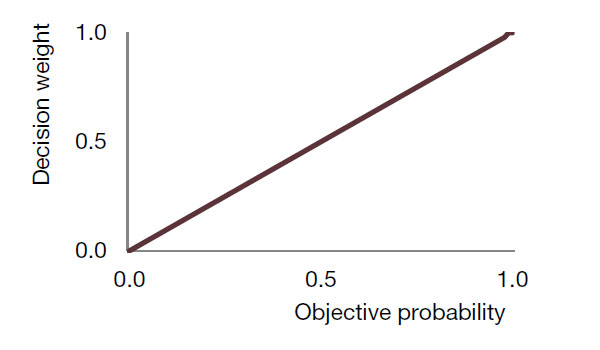
Prospect theory captures the overweighting of tail events with a probability weighting function which transforms actual probabilities into decision weights. A fully rational individual would use the objective probabilities, i.e. would not transform them. But empirical evidence suggests that we do transform probabilities, overweighting low-probability events and underweighting high probability events (see Figure 2). One conjecture is that our evolutionary ancestors used a very crude weighting function that overweighted tail events even more (see Figure 1) and that we are (very slowly) evolving toward the “rational” straight line (Figure 3).

Figure 1: Extreme Decision Weights (possibly our evolutionary ancestor’s weighting function)

​

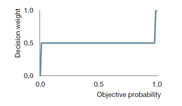
Figure 2: Decision Weights (contemporary weighting function)

​

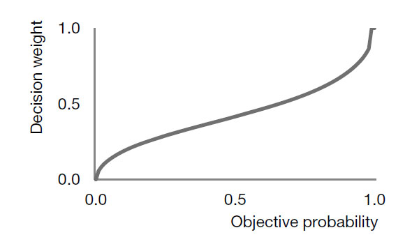
Figure 3: Objective Probability (ideal weighting function)

​

SR: Investors show a strong dislike towards heavily negatively skewed strategies, such as relative value fixed income or buying cat bonds. They don’t seem to mind moderately negatively skewed strategies like Equity Market Neutral. There may be a memory aspect to this. If the tail event is extreme enough, as was the case with LTCM, then it will remain in your memory forever. In contrast, one moves on from a moderately bad event, as we saw with Equity Long-Short in 2007. I’m not convinced investors do explicitly like positively skewed strategies such as buying options. With such a strategy, you spend long periods of time without positive returns.

NB: I see the argument, but the data suggest that investors do like positive skewness – positively-skewed assets typically earn low returns, suggesting that they are highly priced. But this pattern is stronger among smaller-cap stocks, suggesting that it is driven by individual rather than institutional preferences.

SR: People like lotteries. Is it rational to buy a collection of positively skewed instruments?

NB: Economists debate whether we can call a preference irrational. Heavy buying of skewed assets may be defensible so long as buyers know that their expected return is unusually low. If they don’t realize this, then it’s easier to call their behaviour irrational.

CH: One can think of venture capital. It looks a lot like what you expect if skew is risk: positive skew and low average returns. Most venture capital investors are aware of this. It is possible that they believe have a special ability to pick the winners (so the average return is not what they face). It is also possible they understand the average returns are low and they are investing in VC for the positive skew.

 

4. How should skew be priced? Should only the non-diversifiable component of skew be priced, or should idiosyncratic skew also be considered?

CH: For variance, only the asset’s contribution to the variance of a well-diversified portfolio should be priced. This is the so-called systematic risk. However, we find that an asset’s idiosyncratic variance also appears to produce a premium (low volatility effect), which is difficult to explain. For skew, I would say that what should count is how an asset’s skew contributes to the skew of a diversified portfolio. The important measurement then becomes co-skew, which is defined as the component of the asset’s skewness to the market portfolio’s skewness. However, it is possible that idiosyncratic skew could also be priced. Of course, we need some sort of asset pricing model to separate the systematic from the idiosyncratic both for variance as well as skew.

NB: The EU framework predicts that coskewness alone should be priced. But in the PT framework, idiosyncratic skewness can also be priced. There are two ways this can happen. First, in PT, the preference for skewness is so strong that some investors will be willing to take large, undiversified positions in skewed assets. Second, some investors may evaluate their investments on an asset-by-asset basis (so-called “narrow framing”). In both cases, idiosyncratic skewness gets priced.

The evidence suggests that idiosyncratic skewness is indeed priced. We see this in studies of IPOs, distressed stocks, and options, but also in direct tests of the pricing of skewness. More speculatively, there is some recent work that looks at whether cultural differences impact preferences for skew. The idea is that different groups may find the lottery-like payoff associated with skewness more or less attractive. The differences in preferences may be reflected in differential pricing of skewness in different regions.

 

5. Does skewness vary over time or is it intrinsic to an asset? How can we forecast it? Are implied measures useful?

NS: Measuring skew alone is a difficult enough problem due to lack of data, and if one believes it is time-varying than this compounds the complexity. Theoretically, it is very challenging to obtain any kind of single asset model with time-varying skew that is both compelling and stable.

NB: The skewness of a security is affected by many factors, including the economics of the underlying firm’s business, and the identity of the security holders. As a company matures from a young firm to a more established business, its stock’s skewness may change. There is also evidence that the more levered a stock’s holders are, the more negative skewness there is in the stock’s returns, as the stock is more likely to be subject to fire sales during downturns.

MS: Some features of skewness are driven by externals that are obviously time-varying. Skewness in credit is influenced by the availability of cheap money and Federal support. This is dictated by central bank behaviour which is by definition time-varying. NG: When trying to estimate volatility, one obtains better estimates by switching to high-frequency (intraday) data. Is there any value in doing the same with skew, or is the point that you are trying to spot outliers so HF is not going to help?

NS: The information you can extract from HF that is useful for studying asymmetries is to try and understand jumps. You can use HF data to identify and quantify the discontinuity of prices, and compare large falls to large rises. This could lead to information about asymmetries over longer horizons, but not directly to skew (third moment).

CH: We have been talking about time-series skew, which is such a difficult quantity to measure and hence even more difficult to forecast. Instead of going firm by firm and trying to forecast skew, an alternative approach is to work in the cross section. It is possible to fit a regression that explains the cross-section of company skew. Such a regression might include variables like the firm’s leverage (which reflects the optionality of the equity) and measures of implied skew.

 

6. How is the skewness of a single asset related to its volatility? Can we control the skewness of the return from an asset by scaling our position using volatility?

NB: Empirically, at the individual stock level, more volatile stocks are also more skewed. So the negative relationship between volatility and returns may actually reflect a negative relationship between skewness and returns.

NS: In equity markets, we often see falls in prices lead to an increase in volatility – the statistical leverage effect. This can cause negative skewness in returns. However, if you scale your positions with respect to volatility, then you can potentially remove or even reverse the skewness of the unconditional returns.

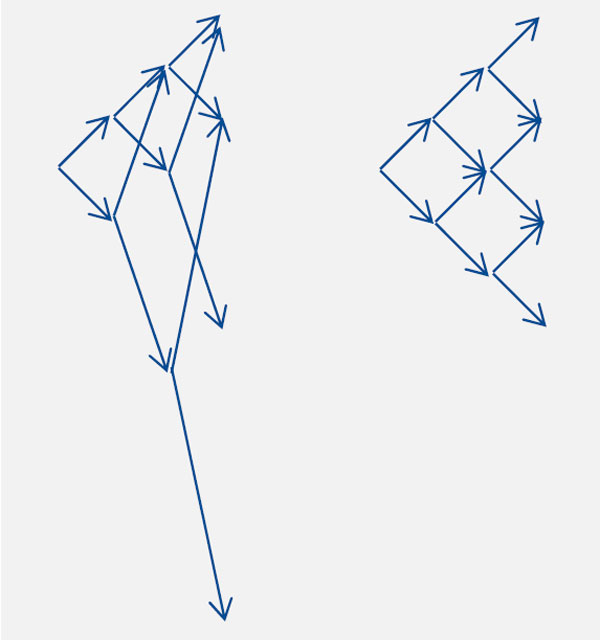
Theoretically, we can demonstrate this using a very simple martingale model. We assume that the price moves up or down by 1 with equal probability, however following a down move the volatility doubles. We then study the return profile after three steps with and without volatility scaling.

In the first setup, we hold a constant position at each point. This leads to a left-tail heavy return profile. In the second setup, we scale our position by halving the size of our exposure following a down-move/increase in volatility. The return distributions of the two approaches can be seen in Figure 4. We observe that the constant position sizing leads to a negatively skewed return, whilst if we volatility-scale we are left with a symmetric return profile.

Figure 4: Return profile: without and with volatility scaling

​

NG: We do this when we construct our momentum systems. By scaling according to both the volatility of the market and your performance, you can construct a positively skewed historical return profile. Effectively, this is a result of the correlation between performance and risk. One can demonstrate this result theoretically under mild assumptions on the underlying.

NS: More generally, one can view a trading strategy as a means of seeking to transform one return distribution to another: the asset’s return distribution to the portfolio’s distribution. In the case of momentum trading, you are taking your asset’s return distribution and returning one with positive skew. Returning to theory, if we model the underlying asset via a martingale, then one can select a trading strategy to produce any desired degree of asymmetry in the return profile.

 

7. How does skewness relate to drawdowns?

CH: Due to the many different meanings of the word skew this makes the question more difficult. Most people believe that negative skew leads to larger drawdowns.

NG: This is theoretically a very interesting problem. In the case of momentum which we can model analytically, we see positive skewness helps lessen drawdowns. More generally than momentum, the problems quickly become intractable analytically. One can work empirically using Monte-Carlo simulations, and doing so one does see a link between skewness and drawdowns.

CH: When modelling drawdowns, the mean of the return distribution is also very important. This makes it difficult to model, and you end up with very large error bars.

SR: We see empirical evidence to support the fact that drawdowns are linked to skew. For clients, drawdowns are of the upmost concern, many in fact use skew as a proxy for drawdowns.

NS: If you were to characterise different investment strategies, one way would be to report expected maximum drawdown over say a 10 year period. This number could be compared to a vanilla strategy. This would provide a more direct means of distinguishing between strategies, rather than intuiting drawdowns from skew/asymmetries in the return distribution. The problem with this approach would be that there are large error bars around forecasting drawdowns, as they are a single observation.

CH: One way to make such a measurement more robust would be to look at in addition to the max drawdown, the second to max, third to max, etc.

GB: In practice, it seems that the best way to minimise drawdowns is to maximise both Sharpe and skew.

 

8. CTA’s returns have been shown to be positively skewed¹. Is it a consequence of the central limit theorem that diversification destroys skewness?

NS: If you have a factor structure to your returns, then constructing a portfolio will place weight on the major common factors. This means that if the returns in the major factor(s) are skewed, then diversification will not destroy skewness as the skewness of the factor(s) will live through.

MS: Empirically you observe a common factor structure across many assets. Equity indices for example are clearly exposed to a “market factor”. It does feel that when you run strategies with positive skew it is relatively hard to knock it out.

NG: There is also some interplay between momentum and correlation. We observe that when assets trend they often become more correlated, which makes the central limit theorem less relevant. This can justify why one observes positive skew from momentum strategies running across a large universes of assets.

 

9. How can we manage skew in a portfolio?

CH: The naïve answer would be to construct a portfolio using some form of mean-variance-skew optimisation. Few do this because the inputs are simply too noisy. If we had a good handle on the expected skew and our utility for it, then skew should be a crucial input for portfolio construction.

NG: We think a lot about this at AHL. One obvious way to help manage the skew of a portfolio is to add an allocation to momentum. This helps to mitigate any negative skewness. Volatility scaling is also very valuable at the model level, as is conditioning models, potentially on momentum, to pull in the left tails. In theory, the central limit theorem should help ensure that a portfolio consisting of many uncorrelated models should not have a negative skew.

CH: When you consider adding a new strategy within AHL do you calculate the co-skew and see its effect?

NG: No. I don’t believe that we can measure this accurately enough.

CH: But you do care about the skew.

NG: We will look at the models, and use both backtests and theory to classify the skew as either positive, negative, or zero. We then work from there.

MS: We also look at co-dependencies in the tails. These are more reliable to measure than co-skew, and we want to be very careful about increasing tail correlations.

GB: Our general approach at Numeric is to try and diversify the signal set whilst being mindful of leverage. To help manage skew in our equity market neutral strategies, we try and roughly allocate equally to value and momentum. We also take into account the crowding of strategies as we believe this can lead to a liquidity event, and hence negative ex-ante skew.

NG: If you have a selection of models that have a low tail correlation, then you can believe that you are managing your skew. However, the added diversification does come at the cost of leverage which itself can potentially introduce negative skew.

 

 

APPENDIX: SKEW - A BRIEF SURVEY

In a mathematical sense, skewness provides a measure of the asymmetry of a probability distribution. In the case of asset returns, which tend to be unimodal, skewness can very roughly be interpreted as the degree to which the right tail is longer than the left (Salkind, 2006).

A serious problem with this measure is that it is extremely sensitive to outliers. As an example of this, (Kim & White, 2004) compute the sample skewness of the S&P 500 using daily returns between 1982 and 2001 - a sample set of 5085 observations. They arrive at the value of -2.39 however if they recompute whilst omitting the single observation relating to the 1987 stock market crash, when the index dropped by -20%, the value changes to -0.26. In order to better estimate asymmetries in return distributions, other more statistically robust methods have evolved. These methods include working with quantiles, studying semi-variance (Feunou, Jahan-Parvar, & Tedongap, 2014), and fitting families of skewed distributions to the dataset (Jones & Faddy, 2003).

Moving on from the question of measuring skewness in return distributions, one can ask whether skew should be priced – i.e. should a skewness premium exist. In traditional pricing models, investors are assumed to evaluate risk according to the Expected Utility (EU) framework. These models predict that a quantity called coskewness will be priced and there is some empirical evidence to support this (Harvey & Siddique, 2000).

Recent research has emerged to suggest that investors evaluate risk not according to EU, but according to a psychologically more realistic framework, namely Prospect Theory. These models predict that an asset’s own skewness will also be priced (Barberis & Huang, 2008). That is a positively skewed asset will be overpriced and earn a lower average return, while a negatively skewed asset will be under-priced and earn a higher average return.

The intuition is straightforward. Prospect theory posits that people overweight low-probability events (this is motivated by the fact that people like both lottery tickets and insurance policies). But if they overweight low-probability events, they are going to have a strong preference for positively skewed assets: they will overpay for such assets and accept a low average return on them. The converse is also true concerning negatively skewed assets: they will underpay for such assets and demand a high average return on them.

This skewness premium has been used to help explain a number of puzzling pricing facts. For example, the return distribution of IPOs in the initial three years has been observed to be positively skewed. Furthermore, the average return by such a company was significantly below a set of comparable firms (in terms of size and industry) (Ritter, 1991). One possible explanation for the skew is that IPOs are conducted by young firms. A large proportion of their value is thus related to future growth, which can be considered an option like quantity. Other examples of positively skewed asset classes earning below average long-term returns include distressed stocks (Campbell, Hilscher, & Szilagyi, 2008), and OTC stocks (Eraker & Ready, 2015).

At the individual asset level, there is the question of how do we forecast skew? Historical skew is an important ingredient in forecasting skew, however on its own it does not appear sufficiently powerful (Boyer, Mitton, & Vorkink, 2009). (Chen, Hong, & Stein, 2001) use a combination of increase in turnover and increase in asset price to forecast negative skew. (Boyer, Mitton, & Vorkink, 2009) also incorporate historical volatility into their forecast of skewness.

Of importance in practical finance is controlling the skew. Volatility scaling in particular can help normalise the return distribution and hence reduce skew. We see empirical evidence to support this in the work of (Andersen, Bollerslev, Diebold, & Ebens, 2001). They study the daily returns of the 30 DJIA stocks between 1993 and 1998. For each name, they compute ex-post volatility estimates using 5-minute intraday returns. They then compare the raw returns, to the volatility scaled returns and observe that the volatility scaled returns closely resemble normal distributions. In particular; the skewness has been significantly reduced. A key requirement to applying these results in practice is the ability to accurately forecast volatility. Significant research has been undertaken to improve volatility forecasting by using high-frequency historical data (Shephard & Sheppard, 2010).

At the portfolio level, it is interesting to note that certain trading styles can also lead to skewed returns even if the underlying assets themselves are not skewed. An example of this is the case of univariate momentum strategies which under mild assumptions on the underlying can be theoretically shown to be positively skewed (Martin & Zou, 2012). Intuitively this happens because trend following has natural stops: it reduces positions when it loses money and builds positions only after locking in a profit. This is corroborated by empirical evidence in the CTA industry.

 

 

WORKS CITED

Andersen, T. G., Bollerslev, T., X, D. F., & Ebens, H. (2001). The distribution of realized stock return volatility. Journal of Financial Economics, 43-76.

Barberis, N., & Huang, M. (2008). Stocks as lotteries: The implications of probability weighting for security prices. The American Economic Review, 2066-2100.

Boyer, B., Mitton, T., & Vorkink, K. (2009). Expected idiosyncratic skewness. Review of Financial Studies.

Campbell, J. Y., Hilscher, J., & Szilagyi, J. (2008). In search of distress risk. The Journal of Finance, 2899-2939.

Chen, J., Hong, H., & Stein, J. C. (2001). Forecasting crashes: Trading volume, past returns, and conditional skewness in stock prices. Journal of Financial Economics, 345-381.

Eraker, J., & Ready, M. (2015). Do investors overpay for stocks with lottery-like payoffs? An examination of the returns of OTC stocks. Journal of Financial Economics, 486-504.

Feunou, B., Jahan-Parvar, M. R., & Tedongap, R. (2014). Which parametric model for conditional skewness? The European Journal of Finance, 1-35.

Harvey, C. R., & Siddique, A. (2000). Conditional skewness in asset pricing tests. The Journal of Finance, 1263- 1295.

Jones, M., & Faddy, M. (2003). A skew extension of the t-distribution, with applications. Journal of the Royal Statistical Society: Series B (Statistical Methodology), 159-174.

Kim, T.-H., & White, H. (2004). On more robust estimation of skewness and kurtosis. Finance Research Letters, 56-73.

Martin, R., & Zou, D. (2012). Momentum trading: skews me. Risk.

Ritter, J. R. (1991). The long-run performance of initial public offerings. The Journal of Finance, 3-27.

Salkind, N. J. (2006). Encyclopedia of measurement and statistics. Sage Publications.

Shephard, N., & Sheppard, K. (2010). Realising the future: forecasting with high-frequency-based volatility (HEAVY) models. Journal of Applied Econometrics, 197-231.

 

1 The Barclay BTOP 50 Index monthly return 1987-2016 has a skewness value of 1.0