Introduction
While machine learning models may have improved returns, investors are currently somewhat blind to where those returns are coming from.
Modern portfolio management has increasingly embraced machine learning (ML) models to predict returns due to their ability to capture complex interactions between factors. The drawback is that the end result is often something close to a black box model with highly optimised outputs. This means it is often challenging to understand a model’s predictions and decision-making. To counter this, model interpretation or attribution techniques are used to attempt to explain the rationale behind model predictions and to uncover the features that contribute most to the outcome. However, little progress has been made so far to leverage ML models for factor portfolio attribution, which is a critical component of systematic portfolio investment. Without this evolution, it is difficult to accurately understand which factors are affecting portfolio returns. While ML models may have improved returns, investors are currently somewhat blind to where those returns are coming from.
Existing linear factor attribution methodologies suffer from limitations such as a lack of ability to capture local interaction effects and the implied assumption of a singular global beta. Instead, we would argue that systematic investors need to look beyond the existing linear attribution models to find granular, local explanations of performance.
One solution is to use Shapley value. In this paper, we delve into what Shapley value is, how it can be applied to explain model outputs, and how we compute Shapley values using SHapley Additive exPlanations (SHAP) – a specific implementation of Shapley value. We also explain how a SHAP based performance attribution framework can be used for local and global portfolio attribution and introduce an innovative portfolio attribution system which uses Shapley value and SHAP to explain both the decision-making process and cross-sectional return variation at a local and global level. We also demonstrate the enhanced explanatory power of SHAP attribution by incorporating non-linear ML models such as XGBoost.
Why Change? The Limitations of Existing Linear Factor Attribution Methodologies
If ML models continue to provide reasonable returns, why worry about refining attribution methodologies? In short, because they are inadequate. Existing factor attribution methodologies such as time series regression, cross-sectional return attribution, and holdings-based attribution are based on linear models, making them unable to capture local interaction effects with the assumption of global linear beta.
For example, time series regression is limited by the dimensionality problem and the assumption of constant beta throughout time, making it less useful for dynamic portfolio management. Conversely, cross-sectional return attribution with a set of risk factors, as commonly used by risk model vendors, assumes that return generation can be attributed to a linear global factor model. Its close cousin, holdings-based attribution, estimates the exposure of the portfolio holdings to a set of custom factor portfolios. Although all three methodologies are based on the same linear factor return structure, they differ in terms of sophistication and customisation flexibility. However, these methodologies are not capable of capturing interaction effects due to the non-linear relationship between those independent variables.
The Solution: Introducing SHAP Portfolio Attribution
The Shapley value is a concept from cooperative game theory that measures the contribution of each player to a coalition game’s payout.
The Shapley value is a concept from cooperative game theory that measures the contribution of each player to a coalition game’s payout. The four axioms of Shapley value1 ensure that the payout distribution is fair when players can form coalitions and payout depends on the coalition’s performance. Shapley value is the only payout method that satisfies these four axioms. Payout distribution is calculated based on the marginal contribution of a player by permutating through all combinations of the players.
The basic idea behind SHAP attribution is to explain every security’s output (weight and return) as the sum of the contribution of each factor (aka feature in ML language). The set of factors used is defined by users. Examples include fundamental factors such as Barra factors, model scores or any metrics that can be used as inputs to a model that help predict the output. The SHAP value for a feature is the change in expected value brought by including that feature. This approach allows us to decouple the attribution from the underlying models used to explain portfolio holdings or stock returns, providing the flexibility to use any model we see fit to explain portfolio weight and cross-sectional returns.
SHAP attribution can capture local interaction effects and other non-linear relationships that are beyond the reach of linear models employed in existing attribution methodologies.
With such an approach, we should be able to explain the decision-making process and cross-sectional return variation for every security in a portfolio i.e. a local explanation. SHAP attribution can therefore capture local interaction effects and other non-linear relationships that are beyond the reach of linear models employed in existing attribution methodologies.
Computing an exact Shapley value is computationally expensive and intractable when the number of features is large. Therefore, an approximate solution is necessary. One such way to compute an approximate Shapley value is through statistical sampling. SHAP is a popular implementation of the Shapley value and provides several approximation algorithms. It includes Kernel SHAP, a model-agnostic implementation of Shapley value and a few fast, efficient model-specific algorithm such as TreeSHAP for computing Shapley values. For all our studies, we use the SHAP package with Python API to compute the approximate Shapley value. Specifically, we use TreeSHAP when underlying models are decision tree based.
SHAP Portfolio Attribution Framework
We propose a portfolio attribution framework based on SHAP implementation of Shapley value. Attribution is the process of explaining the performance of a portfolio. Performance is the sum of product of each security’s weight and return held in the portfolio. Investors have control over the portfolio weights but no control over the return. Therefore, portfolio attribution needs to explain both how investment decisions are made and what drives the returns. In general, investors use their proprietary models and a set of factors (style, industry, or country factors) to explain investment portfolio weights and cross-sectional return variation.
The model-agnostic property of Shapley value allows us to separate the models used to predict the output and the attribution of the factors used to explain the predicted value. Non-linear ML models can be used for explaining both decision-making and cross-sectional return sources. Linear models impose a strict global structure and embed a causality assumption, while non-linear ML models only require correlation and association.
For global interpretation at a portfolio or group level, we can aggregate SHAP values bottom-up from the security’s Shapley values. In addition to consistency between local and global explanation, this approach offers flexibility and customised aggregation.
Illustration of SHAP Attribution Framework
The following diagram shows the framework for SHAP attribution. We fit two models based on user supplied factors, one to explain the decision-making process (i.e. the weight of a security in the portfolio) and one to explain cross-sectional return sources. Empirically tree-based models offer much better explanation, consistent with our observations that non-linear interaction between factors plays a significant role in both investment decision making (as the portfolio is subject to various investment and liquidity constraints even when return forecast comes from linear factor models) and cross-sectional return sources.
Figure 1. Performance Attribution as the Sum of Security Weight Multiplied by Return
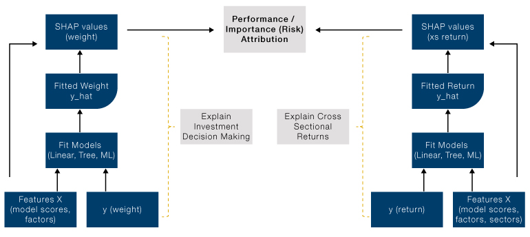
Source: Man Numeric. For illustrative purposes.
Portfolio return is simply the sum of each security’s weight multiplied by its return. Figure 1 shows that the model-fitted weight can be written as the sum of SHAP values of factors used to fit the weight model. Similarly, model predicted return can be written as sum of SHAP values of factors used to fit the return. Therefore, the return attribution for each security is simply the security’s weight SHAP multiplied by its return SHAP – this is a face splitting product in matrix terms. Global performance attribution is done by aggregating SHAP values from security level. It is worth noting Shapley value measures the marginal contribution, which implies that SHAP value for the return is an attribution of excess return when the model is fitted over a broad universe; and for weight, active weight is preferred as it is more consistent with the marginal concept.
Interpretation and Connection to Existing Linear Factor Attribution
In the previous section, we demonstrate a general performance attribution framework using SHAP values to attribution portfolio weight and security return. This leads to the following equation at portfolio level:

If we use m features to explain weight and k features to explain return, there will be m*k SHAP values to explain the performance of each stock as a result of the full expansion. If the residual, which is the difference between the model-explained value and the true value, is also included in the calculation, then there are (m+1)*(k+1) performance attribution items for each security. This can become unwieldy and uninterpretable, even with a small number of features, and therefore some aggregation is needed. This framework offers users full control of how data should be aggregated and interpreted. We suggest two intuitive approaches and highlight their connection to existing linear factor portfolio attribution:
- Aggregating from the weight side - for each feature in the m features used to explain the weight of a security, the k values used for returns are added up. With this aggregation method, there are m SHAP values to explain the performance of each security.
- Aggregating from the return side - for each feature in the k features used to explain the return of a security, the m SHAP values used for weight are added up. With this aggregation method, there are k SHAP values to explain the performance of each security.
One benefit of the full expansion of weight and return SHAP values is to answer questions such as, for stock A, how much contribution comes from the weight driven by the Momentum factor and the return of the stock due to the Value factor? This is stock A’s weight SHAP for Momentum multiplied by its return SHAP for Value. We can roll up this term across all securities to get a portfolio level answer.
Figure 2 illustrates the two methods. In this stylised example, Value is used to explain both weight and return, and the aggregation is done from either weight (grey lines) or return (yellow lines) side. We end up with very different explanations for how much performance we can attribute to Value. We would like to point out that attribution from the weight side is equivalent to the holdings-based attribution (HBA) when the underlying weight model is linear (with residual in security return included). Attribution from the return side is equivalent to the cross-sectional return-based attribution when the underlying return model is linear (with residual in weight included). Conceptually, the SHAP attribution we propose here is a more general framework that can accommodate the current factor attribution methods.
In this general framework, we have reconciled the often puzzling empirical observation that the same factor can have very different attribution using HBA versus returns-based attribution. Contrary to some claims, there is no inherent advantage of HBA over return-based attribution. They are both global linear model-based explanations with different perspectives; one uses factors to explain weight decision and ignores the return sources and the other approaches from the return side and ignores the drivers for investment decisions. Depending on the use case, one of the two aggregation methods may be preferred over the other, or sometimes interaction terms may also be of interest – as demonstrated by our previous example using Momentum as the weight source and Value as the return source. We can see in the diagram that the total “explained” performance remains unchanged no matter from which side we aggregate. We leave out the residual which is the “unexplained” part, and thus is one of the insights offered by the SHAP attribution framework.
Figure 2. Two Methods of Performance Attribution
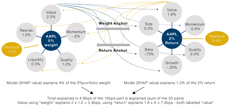
Source: Man Numeric. For illustrative purposes.
Enhanced Explanatory Power with SHAP and XGBoost
It should be noted that tree-based models have the tendency to “overfit” the data compared to linear regression, so regularisation is important to balance the additional explanatory power against overfitted, nonsensical results. Overall, the enhanced explanatory power and flexibility of SHAP attribution enable us to improve our understanding of portfolio management and investment decision-making at the most granular level.
Conclusion
Portfolio performance attribution is crucial in understanding and trusting the investment process.
Portfolio performance attribution is crucial in understanding and trusting the investment process. It is a challenging task for systematically managed portfolios as the “black box” nature of the models and the highly optimised portfolio construction make the output less interpretable. Shapley values combined with non-linear ML models are powerful tools for interpreting black box models and understanding model or factor contributions, providing insights into the decision-making processes, and realised return sources. Finally, the technique used here may offer potential research areas beyond performance attribution, such as the possible construction of risk models with embedded non-linearity using SHAP values for cross-sectional returns.
1. The four axioms include: efficiency, nullity, symmetry and additivity.
You are now leaving Man Group’s website
You are leaving Man Group’s website and entering a third-party website that is not controlled, maintained, or monitored by Man Group. Man Group is not responsible for the content or availability of the third-party website. By leaving Man Group’s website, you will be subject to the third-party website’s terms, policies and/or notices, including those related to privacy and security, as applicable.