Factors

Acknowledgements

Edward is grateful to Cam Harvey and Otto Van Hemert for comments.

1. Introduction

In classical finance, a factor is a source of undiversifiable risk. Since we shall be loose with our definition of ‘factor’ in what follows, we refer to classical factors as risk factors. Portfolios exposed to a risk factor should earn a risk premium for bearing the factor’s undiversifiable risk, resulting in higher expected returns than otherwise. The undiversifiable risk could, for example, be variance attributable to the market portfolio (i.e. market beta), negative skewness, illiquidity, or sensitivity to macroeconomic surprises such as unexpected inflation and growth shocks. Importantly, from this aspect, a risk factor is not necessarily tradeable.

Figure 1. Growth in Factor ‘Discovery’

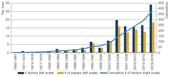
As published in top academic journals through to the end of December 2018. Reproduction of a chart of Harvey and Liu (2019).

More recently, factors have been constructed in stock markets by building long-short portfolios of stocks where positions are sized with reference to a particular firm characteristic: for example, P/E ratio or market capitalisation. The origin of this approach was to build portfolios that acted as proxies for risk factors (see Fama and French (1993)). The problem of risk-factor identification has shifted to the identification of firm characteristics that can be used to construct portfolios with high returns. The reasoning is that high returns imply the presence of a risk premium, and therefore risk-factor exposures. This is possibly a roundabout argument to the finance theorist. Daniel and Titman (1997) provide further discussion on this topic, and provide evidence that the higher returns of value and size portfolios are not due to risk-factor exposures. We note that the link between high returns and risk premia is a tenuous one. High returns could be due to luck or mispricing, rather than risk-factor exposure.

From an investment perspective, the portfolio approach to factor construction is helpful since the factors are effectively out-of-the-box trading strategies. An investor will want to avoid lucky factors; luck runs out. The investor may be happy with mispricing factors, assuming that the mispricings are not completely arbitraged away in future. The portfolio approach has also led to an explosion of academic interest in characteristic identification for factors, which is demonstrated by the chart of Harvey and Liu (2019) reproduced in Figure 1.

The purpose of this introduction is not to fix a particular view of what a factor is, but to provide a lens through which to view factors in general. We are primarily interested in tradeable factors, whether exploiting mispricings or providing proxies for risk factors. In general, when discussing factors, the link back to risk factors is sometimes overlooked, but should not be.

2. Factors

We define factors to be investment styles with positive expected returns: in the long run, they deliver positive returns to those willing to bear risk, or those able to identify and exploit mispricings. Some factors are static, in the sense that they can be captured by buy-and-hold portfolios (or at least portfolios with very low turnover): for example, the equity risk premium and the term premium. Other factors are dynamic, requiring active trading to capture effectively: for example, the equity value factor and the equity momentum factor, although one might expect a value portfolio to turnover more slowly than a momentum portfolio. Various theories of factor investing postulate that much of the variation in the returns of a large portfolio of assets can be explained by the portfolio’s exposure to a small number of factors.

This description of factors given in Ang (2014) focuses more on risk factors and their proxies:

"Factors are investment styles that deliver high returns over the long run. The risk premiums don’t come for free, however, as factors can underperform in the short run (‘bad times’). Factor losses are associated with bad economic outcomes, like times of high inflation and slow economic growth. Equities and bonds are examples of factors whose risk premiums are obtained by simply buying assets (long-only positions), hence they are static factors. Other factors require dynamic trading involving long-short positions, where we constantly have to adjust portfolio weights. Just like their static factor cousins, dynamic factor strategies – like value-growth investing, momentum and short volatility strategies – don’t always make money, and investors have to brace for stomach-turning stumbles. It is precisely for suffering these losses that factors accrue risk premiums. Assets embed different combinations of factor risks, just as foods mix different types of nutrients."

Ang (2014) also provides the following list of criteria that should be met when considering a factor for investment (text in bold is repeated verbatim, see also Ang et al. (2009)):

1. Be justified by academic research: We require economic or behavioural justification for the risk premium, and strong empirical evidence of the risk premium;
2. Have exhibited significant premiums that are expected to persist in the future: We must justify a belief that the factor will continue to offer high returns. That is, we expect the risk or behavioural traits that give rise to the performance to persist, despite widespread knowledge of the factor’s existence and competing attempts to harvest it;
3. Have a history available for bad times: To assess properly the risk-return trade-off arising from investing in a factor, we need to understand the severity of potential bad outcomes;
4. Be implementable in liquid, traded instruments: Scalability is an important consideration for large investors. Also, dynamic strategies are often implemented as long-short strategies, and require leverage to achieve desired levels of returns or volatility.

Note that point 4 excludes certain macro factors (such as business-cycle indicators) and latent factors extracted from ex-post statistical techniques. While such factors have important roles to play in investment and risk management, they fall out the scope of our discussion, beyond the following remarks. Chen et al. (1986) provide evidence that stock price sensitivity to macroeconomic innovations earns a risk premium. In an international study, Liew and Vassalou (2000) show that value and size factors – but not momentum – contain information about future economic growth. This provides empirical support to the view that value and size are risk factors.

2.1. CAPM

Based on the theory of portfolio selection from Markowitz (1952), the Capital Asset Pricing Model (‘CAPM’) developed in the 1960s (see Treynor (1961, 1962), Sharpe (1964), Lintner (1965) and Mossin (1966)) is a single-factor model of equity returns: the single factor being the market portfolio. In the CAPM, the expected excess return of a stock is equal to its market beta times the expected excess return of the market portfolio. A stock’s idiosyncratic risk carries no premium.

The assumptions of the CAPM are strong and its predictions have been overwhelmingly rejected by empirical evidence (see, for example, Fama and French (1993)). As early as 1970, Friend and Blume presented a negative relationship between stock returns and beta. On the other hand, Black et al. (1972) and Fama and MacBeth (1973) find a positive relationship between stock returns and beta, but find that it is flatter than predicted by the CAPM. However, they are not able to reject the model of Black (1972), a variation of CAPM with borrowing restrictions.

2.2. Multi-Factor Models

The Arbitrage Pricing Theory (‘APT’) of Ross (1976) provides a framework for describing the returns of assets in terms of multiple risk factors. In particular, in APT, the expected excess return of asset i can be written:

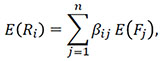
where F _j is the excess return of one of n factors.

Also related is the intertemporal capital asset pricing model (‘ICAPM’) of Merton (1973). In this continuous-time model, investors maximise their expected utility. The model includes state variables that form factors alongside the market portfolio.

Sharpe (1982) presents some regression methods for the ex-post identification of multiple factors. He applies the methods to US stocks to examine value and size effects, among others.

Importantly, the identification of factors (besides the market portfolio) is a rejection of the CAPM.

3. Stocks

Providing sufficient evidence of positive expected returns makes the identification of dynamic stock factors tricky, to say the least. As mentioned, ex-post high returns could be due to luck, rather than risk premia or mispricings. This is something that we shall return to later.

3.1. Value

Perhaps the oldest dynamic equity factor is the value factor. The principles of value investing have long been documented (Graham and Dodd, 1934), but it was Basu (1977) who showed that stocks with low P/E ratios (cheap stocks) outperformed stocks with high P/E ratios (expensive stocks).

The P/E ratio is just one of dozens of value metrics that have been proposed for the construction of value factors.

Value factors have suffered drawdowns (although not as deep as the market portfolio or momentum), and performance recently has been weak, which can be seen in Figure 2. Taylor et al. (2018) provide commentary on the recent performance of, and the outlook for, value investing. They identify two broad environments that have been particularly challenging for value. Firstly, periods of weakening economic growth, which is possibly related to an increase in investor risk aversion. The second environment is a growth-driven market where firms’ prospects are being over-extrapolated.

Figure 2. Fama and French’s Three Factors

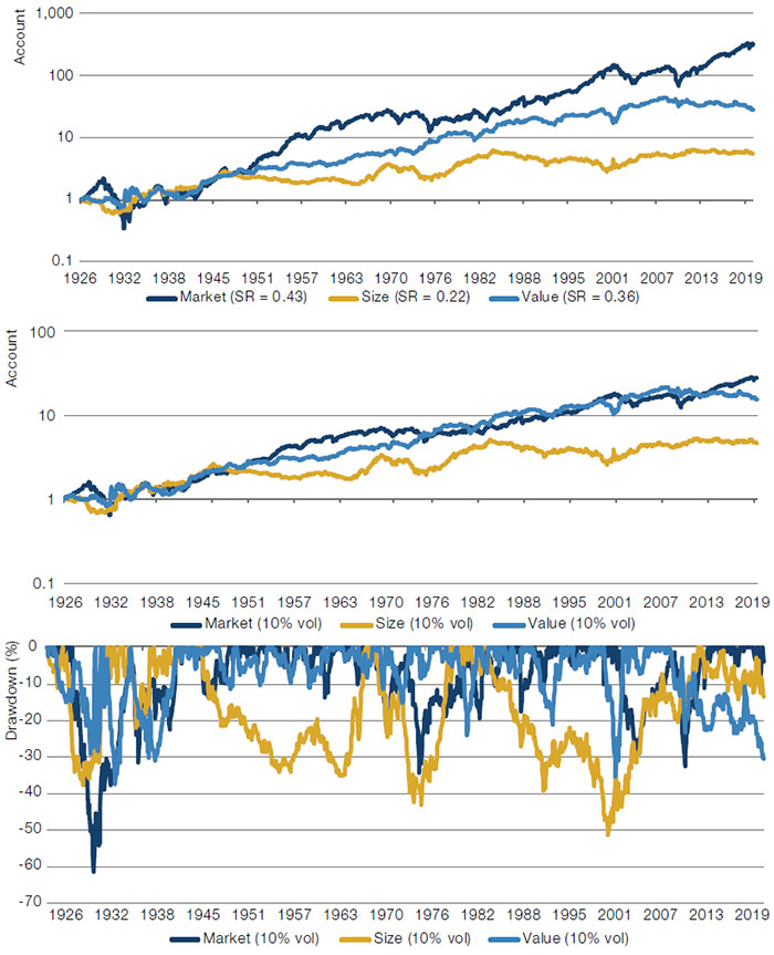
The three US equity factors of Fama and French (1992) using data from French’s website. Sharpe ratios are given in parentheses in the top legend. Middle chart shows performance after ex-post scaling to 10% volatility. Bottom chart shows draw-downs at 10% volatility.

The value factor may be a proxy for a fundamental risk factor. Fama and French (1993) explain:

"Not surprisingly, firms that have high BE/ME (a low stock price relative to book value) tend to have low earnings on assets, and the low earnings persist for at least five years before and five years after book-to-market equity is measured. Conversely, low BE/ME (a high stock price relative to book value) is associated with persistently high earnings."

The value factor may also benefit from mispricing due to behavioural traits. Lakonishok et al. (1994) find evidence that market participants consistently overestimate growth rates for ‘glamour stocks’ relative to value stocks.

3.2. Size

Banz (1981) first identified a ‘size effect’ in US stocks, where stocks with a small market capitalisation exhibited higher risk-adjusted returns than stocks with a medium or large market capitalisation. The size factor then takes long positions in small stocks and short positions in large stocks.

Fama and French (1992) identified the importance of combining value and size to explain the cross-section stock returns. The same authors then constructed value and size factors in Fama and French (1993), which – combined with the market portfolio – form their influential 3-factor model of stocks returns. In this case, double sorting was implemented to reduce any influence of value on the size factor.

The size factor has not been without its critics. Notably, Black (1993) points out the poor post-publication performance of the size factor (see Figure 2), and questions whether the results of Banz (1981) are partly a result of data mining – a question that continues to recur in the world of empirical asset pricing.

More recently, Asness et al. (2018a) have argued the case for size, emphasizing the need to adjust for bias due to exposure to the quality factor, which we shall come to later.

It is difficult to motivate the size factor as a proxy for a risk factor. However, Fama and French (1993) note “the fact small firms can suffer a long earnings depression that bypasses big firms suggests that size is associated with a common risk factor that might explain the negative relation between size and average return.”

3.3. Cross-Sectional Momentum

Jegadeesh and Titman (1993) show that stocks with higher recent returns outperform stocks with lower recent returns. The momentum factor is constructed by buying past winners and selling past losers. Although prone to nasty crashes, the momentum factor continued to perform post-publication.

Carhart (1997) added momentum to the 3-factor model of Fama and French (1993) for US stocks. Fama and French (2012) provide an international study of this 4-factor model. This model has become the workhorse of academic asset pricing in equities.

Momentum is another phenomenon that is difficult to motivate from economic theory. Behavioural explanations are the most broadly accepted, pointing to investors under- and overreacting to news (see Barberis et al. (1998), Daniel et al. (1998), Hong and Stein (1999), and Hong et al. (2000)). This provided the topic of a previous Academic Advisory Board Meeting (Barberis et al., 2014).

Lou (2012) finds that stock momentum is partially explained by flows into US mutual funds. Well-performing mutual funds attract inflows at the expense of poor-performing funds. This leads to the buying of stocks in the better-performing funds, and the selling of stocks in poor-performing funds. As well as offering an explanation for persistence in mutual fund performance, this mechanism is also a potential source of stock momentum. By similar reasoning, flows might explain momentum in factors themselves, which links to factor timing (see Section 8).

3.4. Illiquidity

Pástor and Stambaugh (2003) estimate an aggregate market exposure to illiquidity, and rank stocks by their sensitivity to this measure. They find that stocks with a greater sensitivity to the illiquidity measure have higher returns. That is, they find evidence for an illiquidity premium in stocks. The illiquidity factor can then be constructed by taking long positions in stocks with the highest sensitivity to the liquidity measure, and short positions in stocks with the lowest sensitivity.

Amihud et al. (2005) provide a survey of illiquidity as a risk factor. They explain that an illiquid asset commands a relatively lower price since

"...the required return is the return that would be required on a similar security which is perfectly liquid, plus the expected trading cost per period, i.e., the product of the probability of trading by the transaction cost."

3.5. Skewness

Kraus and Litzenberger (1976) extend CAPM to include skewness as a risk factor. In their model, a stock’s expected excess return is a linear function of both its covariation and coskewness with the market portfolio. In empirical tests of the model, the authors infer that investors have an aversion to variance and a preference for positive skewness.

Harvey and Siddique (2000) develop a conditional version of Kraus and Litzenberger’s model. For US stocks, the authors find that coskewness is an important risk factor, even after controlling for size and value. They also present a link to momentum, observing that portfolios of past winners have higher returns but lower skewness than portfolios of past losers. The authors motivate the existence of a skewness risk factor with utility theory:

"Everything else being equal, investors should prefer portfolios that are right-skewed to portfolios that are left-skewed. This is consistent with the Arrow-Pratt notion of risk aversion. Hence, assets that decrease a portfolio’s skewness (i.e., that make the portfolio returns more left-skewed) are less desirable and should command higher expected returns. Similarly, assets that increase a portfolio’s skewness should have lower expected returns."

Skewness was the topic of a previous Academic Advisory Board Meeting (Barberis et al., 2016).

3.6. Defensive

We present three examples of defensive factors: the quality factor, the low-volatility factor and the low-beta factor. Although the low-beta and low-volatility factors sound very similar, Ang (2014) constructed a version of each and found them uncorrelated, leading him to argue that they are distinct. On the other hand, Novy-Marx (2016) argues that the performance of low-volatility and low-beta factors can be explained by controlling for profitability (quality), size and value – but not vice versa.

3.6.1. Quality

Novy-Marx (2013) provides evidence that profitable firms generated significantly higher average returns than unprofitable firms. Fama and French (2015) add profitability and investment factors to their 3-factor model to create a 5-factor model for US stocks. The investment factor favours firms with low investment (conservative) over those with high investment (aggressive). Over their sample period (1963–2013), the authors find that the additional two factors render the value factor statistically redundant.

Extending these results, Asness et al. (2018b) identify quality (antonym junk) firms based on the desirable characteristics of profitability, growth and safety (they also consider an explicit payout characteristic in their appendix). On average, the stock prices of quality firms are shown to be higher than those of junk firms, but not by a large amount, and quality stocks have provided higher risk-adjusted returns. The authors construct a quality factor by taking long positions in the stocks of quality firms and short positions in the stocks of junk firms.

There is a flight-to-quality effect associated with the quality factor: high-quality stocks tend to outperform junk stocks during periods of market distress. This was noted by Asness et al. (2018b) and further explored by Harvey et al. (2019), who show that quality factors performed well during equity draw-downs (see Figure 3, which is reproduced from their paper).

Asness et al. (2018b) find evidence that stock analysts systematically underestimate the future returns of quality stocks relative to junk stocks. This points to mispricing being a source of returns for the quality factor.

3.6.2. Low-Beta

Frazzini and Pedersen (2014) construct a low-beta factor (which they term a ‘betting against beta’ factor (‘BAB’)). This factor takes leveraged long positions in low-beta stocks and short positions in high-beta stocks. Leverage is employed to construct a beta-neutral portfolio that is able to exploit security market lines that are flatter than the CAPM would imply (Black et al., 1972). Even within the framework of Black (1972), a positive excess return can be earned in this way if a particular investor’s funding constraints are looser than the average. As well as constructing factors for various regional equity markets, Frazzini and Pedersen (2014) also create factors for Treasury bonds, corporate bonds, and a range of futures, forwards and swaps markets.

Figure 3. Performance Over Drawdown Periods

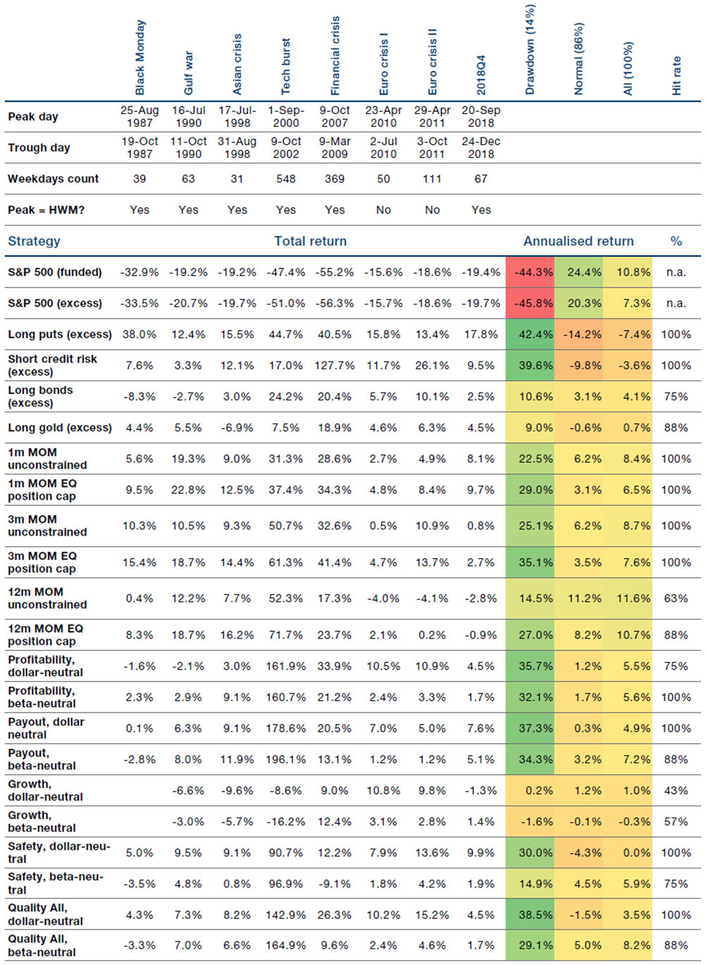
Reproduced from Harvey et al. (2019). The authors report the total return of the S&P 500 and various strategies – including some quality factors – during the eight worst draw-downs for the S&P 500, the annualised (geometric) return during draw-down, normal, all periods, and the hit rate (percentage of drawdowns with positive return). The annualised standard deviation ranges between 6.4% for bonds to 16.5% for the S&P 500, with dynamic strategies all scaled to 10%. The row ‘Peak = HWM’ indicates whether the index was at an all-time high before the draw-down began. The data are from 1985 to 2018. Please see the appendix for additional information on strategy composition.

Novy-Marx and Velikov (2018) remark on various methodological choices by Frazzini and Pedersen (2014), particularly those that deviate from standard approaches, and show that they materially influence the performance of BAB. The authors also point out that BAB overweights very small stocks. When they introduce transaction costs, they find that the returns of BAB are only fair compensation for exposures to investment and profitability factors.

Explanations for the low-beta factor include: (i) mispricing due to demand for high-beta stocks from leverage-constrained investors; and (ii) bearing the risk of forced de-leveraging if funding constraints tighten.

3.6.3. Low-Risk

As mentioned before, Friend and Blume (1970) found some negative relationships between risk and returns in stocks. Haugen and Heins (1975) found related results, and stated:

"The results of our empirical effort do not support the conventional hypothesis that risk – systematic or otherwise – generates a special reward. Indeed, our results indicate that, over the long run, stock portfolios with lesser variance in monthly returns have experienced greater average returns than their ‘riskier’ counterparts."

Ang et al. (2006) ranked stocks by total volatility and idiosyncratic volatility. In both cases stocks with low volatility outperformed stocks with high volatility. The result is even stronger when comparing Sharpe ratios of stocks bucketed by volatility.

Motivation for the low-risk factor is similar to that for the low-beta factor.

3.7. Calendar

In this subsection, we discuss calendar effects in the returns of assets. By calendar effects, we refer to predictability in asset price returns (time-series or cross-sectional) due to periodicity or other characteristics identifiable by dates and times, such as public holidays. Evidence of calendar effects has been widely documented and the range of phenomena is broad. Calendar effects at different frequencies can have low correlation with each other (Keloharju et al., 2016), so it is difficult to define a single, representative factor that captures the essential ingredients of all. We content ourselves by listing a few, differentiating between effects with fixed and variable directionality:

1. Examples of fixed-directionality effects (see, for example, Thaler (1987a,b), Chari et al. (1988), Jegadeesh (1990), Hawawini and Keim (1995), Bouman and Jacobsen (2002), Kamstra et al. (2003), and Swinkels and van Vliet (2012)):
   • January effect: Stocks perform strongly in January, particularly last year’s losers;
   • Weekend effect: Stocks perform poorly over the weekend;
   • Halloween effect: Stock returns are lower in the period May-October than for the rest of the year;
   • Turn-of-month effect: Stocks earn most of their returns in the early part of calendar months;
   • Holiday effect: Stocks earn high returns just before public holidays;
   • Intraday effect: Stocks earn high returns at the starts (except Mondays, due to the weekend effect) and ends of trading sessions;
   • Events: For example, stocks generating positive abnormal returns around earnings announcement dates.
2. Examples of variable-directionality effects (see, for example, Jegadeesh (1990), Heston and Sadka (2008), Heston et al. (2010), Keloharju et al. (2016), Lou et al. (2019), and Baltussen et al. (2019)):
   • Calendar months: Positive correlation between returns of an asset in a given calendar month to returns in the same months in prior years;
   • Intraday persistence: Positive correlation between returns of an asset at particular times of the day, including market open to close and market close to open.

In addition, Heston and Sadka (2008) note that exploiting the seasonality of returns requires trading strategies with high turnover, so transaction costs become an important consideration. Swinkels and van Vliet (2012) find that the Halloween and turn-of-month effects render the January, weekend and holiday effects redundant. Keloharju et al. (2016) state:

"Our results suggest that seasonalities are not a distinct class of anomalies that requires an explanation of its own – rather, they are intertwined with other return anomalies through shared systematic factors."

Heston et al. (2010) postulate that some intraday patterns are caused by systematic investors and institutional fund flows. Lou et al. (2019) state that “essentially all of the abnormal returns on momentum and short-term reversal strategies occur overnight while the abnormal returns on other strategies occur intraday and that this pattern is not driven by news.”

4. Bonds

4.1. Corporate Bonds

Given the vast literature on empirical asset pricing in the stock markets, it is perhaps surprising how small the literature is in the corporate bond markets (the paucity of high-quality data is certainly partly responsible).

Fama and French (1993) use measures of the term premium and credit spreads as factors to explain the returns of portfolios of US government and corporate bonds. Interest in the topic has latterly been reignited, and we mention three recent contributions that construct and test multiple factors. But first, we consider why corporate bonds might need a different set of factors than equities. Israel et al. (2018) provide the following three reasons why corporate bond prices may not track equity prices one-to-one (wording is very close to their own):

1. The fundamental values of bonds and equities depend on the underlying value of the firm’s assets. However, they have differing sensitivities to changes in these assets;
2. Equity and bond values can change even when the underlying value of the firm business does not. They give the example of leveraged buyouts, which tend to benefit shareholders at the expense of debtholders;
3. Bonds and equities are traded in different markets and are typically held by different investors. Stock and bond valuations may diverge, as they are anchored to the risk aversion, liquidity demands and sentiment of different groups of investors.

Houweling and van Zundert (2017) present four dynamic factors of corporate bonds (both long-only and long-short versions of each):

1. Size: long the bonds of firms with small total public debt;
2. Low-risk: long high-rated, short-dated bonds (short positions, when taken, are in low-rated, long-dated bonds);
3. Value: fair-value credit spreads are estimated by regression on rating, time-to-maturity and 3-month spread change. Take long positions in bonds with high actual/fair-value spread ratios;
4. Momentum: long bonds with high trailing 6-month returns (excess of duration-matched Treasury bonds) with 1-month lag for implementation.

Israel et al. (2018) also present four dynamic factors, extending the multi-asset style investment framework of Asness et al. (2015):

1. Carry: long bonds with high option-adjusted spread;
2. Defensive: long bonds based on low firm leverage (net debt as a proportion of net debt plus market capitalisation), high firm gross profitability and low bond duration;
3. Momentum: long bonds based on high trailing 6-month bond returns and high trailing 6-month returns of firm’s equity;
4. Value: long bonds with high spread/default-risk ratios. Default risk is estimated in two ways: (i) a Merton structural model; and (ii) a model based on credit rating, bond duration and bond-return volatility.

Finally, Bektić et al. (2019) present four dynamic factors based on the 5-factor equity model of Fama and French (2015). In this case, the authors use firm characteristics previously used to select stocks to select instead corporate bonds:

1. Size: long the bonds of firms with small market capitalisation of equity;
2. Value: long the bonds of firms with high book-to-market ratio of equity;
3. Profitability: long the bonds of firms with a high ratio of earnings (before taxes) to book equity;
4. Investment: long the bonds of firms with a low growth rate in total assets. The results of their analysis was mixed, with all factors generating significant excess returns in the US high-yield market, but this was not the case for US or European investment-grade markets.

4.2. Government Bonds

Brooks and Moskowitz (2017) propose the following three dynamic factors for government bonds:

1. Value: long bonds with high real yields (nominal yield minus duration-matched inflation expectations);
2. Momentum: long bonds with high trailing 12-month returns;
3. Carry: long bonds with steep yield curves (bond yield minus local short rate).

Brooks et al. (2018) added a fourth, defensive factor to these, which takes long positions in bonds with lower effective duration.

5. Cross-Asset

Although much of the empirical asset pricing literature has been focused on stocks, more generalised approaches have been proposed to apply style investing across asset classes.

Moskowitz et al. (2012) examine time-series momentum in 24 commodity futures, 12 currency forwards, nina equity index futures, and 13 government bond futures. Their principal momentum signal is the sign of the trailing 12-month return of an asset. They find a positive gross Sharpe ratio from time-series momentum in every single asset. They also find that a cross-asset time-series momentum strategy is closely related to a cross-sectional (ranking) cousin, but that it is not fully captured by the cross-sectional approach.

Asness et al. (2013) study value and momentum together, noting that – outside of equities – they are usually considered separately. Given that they find high returns for value and momentum strategies, but a negative correlation between them, it is natural to consider them together. The authors consider four regional equity markets (US, UK, Europe and Japan), and four asset classes (country equity indices, government bonds, currencies and commodities). The momentum measure they consider is the asset price return over the past 12 months, skipping the most recent month. Skipping the most recent month avoids the stock reversal effect documented by Jegadeesh (1990). Skipping has a negative impact for some asset classes, but was applied unilaterally for consistency. The value measures used vary by asset class:

• Single stocks: book-to-market ratio;
• Equity indices: aggregated book-to-market ratio for each country;
• Currencies: average log return of the CPI-adjusted spot price over the last 4.5-5.5 years (i.e. 5-year change in purchasing power parity);
• Commodities: average log return of the spot price over the last 4.5-5.5 years;
• Government bonds: negative of the 5-year change in the 10-year yield.

Cross-sectional value and momentum factors are constructed for each stock region and asset class using a weighted ranking approach (dollar-neutral).

Koijen et al. (2018) examine carry in 13 equity index futures, 20 currency forwards, 24 commodity futures, 10 global bonds, 10 US Treasury bonds with maturities between one and 10 years, intermediate and long-term corporate bond indices, and options on 10 US stock indices. The relationship of carry to value and momentum varies across asset classes. In equities, carry is positively related to value. In fixed income and commodities, carry is positively related to momentum. Across the US Treasury curve, in currencies, in credit and in index options, carry is unrelated to either value or momentum. However, despite any relationships between styles, the authors find that carry returns cannot be completely explained by value and momentum. The the carry measures used by asset class are:

• Currency forward: the difference between the foreign and the local interest rates;
• Equity index future: slope of the futures curve (measured between spot and one-month constant maturity prices);
• Commodity future: slope of the futures curve (measured between the prices of the front two contracts);
• Bonds: a measure that is well approximated by the 10-year yield minus the risk-free rate, plus a roll-down term. When considering US bonds across maturities, this measure is divided by duration;
• Corporate bond index: as US Treasury bonds, using the average yield and duration of bonds in the index;
• Equity index option: a measure that is well approximated by the expected time decay (theta bleed) plus roll-down of the implied volatility term structure (dependent on vega).

For most of the analysis, portfolios are formed within asset classes using a weighted ranking method (dollar-neutral). Time-series strategies are also considered where a long or short position is taken in an asset dependent on the sign of its carry. In either case, carry is found to predict returns across asset classes.

However, in times of global recession or liquidity crisis, carry returns can be poor across asset classes.

As mentioned earlier, Frazzini and Pedersen (2014) construct low-beta factors across asset classes. As well as US single stocks, they consider international single stocks (pooled and by country), US Treasury bonds across maturities, country equity indices, country bond indices, credit indices (by maturity and by rating), commodities and currencies. Factors are formed on a beta-neutral basis. Results show that “betting against beta” generates excess returns across asset classes.

Asness et al. (2015) combine many of the above ideas to form a framework for investing in styles across asset classes. They consider both single stocks and industries within the US, the UK, Europe and Japan; 16 country equity indices; 16 currencies; six government bond futures; five interest rate futures; and eight commodity futures. The authors construct value, momentum, carry and defensive factors across asset classes, and emphasize their high returns and diversification benefits. The factor style characteristics they use can be summarised as:

• Stocks: BE/ME for value, 12-month return (with and without skipping the most recent month) for momentum, and beta for defensive;
• Industry equities and country equities: BE/ME for value, 12-month return for momentum, and beta for defensive;
• Country bonds: real yield for value, 12-month return for momentum, 10-year yield minus 3-month bill yield for carry, and beta to GDP-weighted average for defensive;
• Interest rate futures: real yield for value, 12-month return for momentum, and 3-month roll-down for carry;
• Currencies: real exchange rate for value, 12-month return for momentum, and 3-month cash rate for carry;
• Commodities: 5-year reversal for value, 12-month return for momentum, and slope of the futures curve for carry.

Note that they do not consider carry in equities since it is deemed too similar to value, and they do not define defensive strategies in interest rate futures, currencies, and commodities “because it is difficult to apply the low-beta or quality concepts in these markets”.

Baltussen et al. (2019) replicate several style factors, across asset classes, that have been proposed in the literature, using a long sample period (up to 217 years). The authors are particularly interested in checking the robustness of style factors using out-of-sample data, with a view to assessing whether p-hacking influenced their original proposals. The investment styles analysed are time-series momentum, cross-sectional momentum, value, carry, seasonality and low-beta. The asset classes considered are equity indices, government bonds, commodities and currencies. The authors find evidence supporting most of the style factors. They found little performance decay between their replication sample and out-of-sample periods. They also found that factor returns were present across macroeconomic regimes, and could not be explained by macroeconomic risk.

Baz et al. (2015) compare style investing on a time-series basis with a cross-sectional basis. The investment styles considered are value, carry and momentum, while the asset classes are equity indices (26), currencies (31), commodity futures (16) and interest rate swaps (14). For cross-sectional factors, within an asset class, assets are ranked by their style measures, and long positions are taken in the top six assets versus short positions in the bottom six. For the time-series factors, assets are given an equal weight within asset classes, with the direction (long or short) of an asset’s position determined by the sign of its style characteristic. The authors find that: (a) value worked well in cross section, but poorly in time series; (b) carry worked well in both cross section and time series; and (c) momentum worked poorly in cross section, but well in time series.

Amihud et al. (2005) survey the literature on illiquidity risk, giving examples from studies of government bonds, corporate bonds, inflation-linked bonds, options, hedge funds and closed-end funds.

Lempérière et al. (2017) analyse a wide range of ‘risk premia’ strategies across asset classes (stocks, credit, currencies and equity volatility). Some of these strategies are typical examples of negatively skewed strategies: for example, currency carry and short volatility. They find a negative relationship between the Sharpe ratios of the strategies and their skewness. Time-series momentum provides an interesting outlier, generating significant returns, but with positive skewness. The authors also mention the potential to diversify away some of the skewness by combining strategies.

6. Hedge Funds

We briefly touch upon some factors that have been proposed to explain the returns of hedge funds.

Fung and Hsieh (2004) offer a 7-factor model. The authors have been a driving force behind the academic analysis of hedge-fund and CTA returns. This paper draws from several earlier studies, many by the same authors. Their focus is on hedge-fund indices and funds of hedge funds, which justifies their use of a broad range of factors, since these indices include – for example – equity long-short funds, CTAs and fixed-income hedge funds. Their chosen factors are:

1. The equity market portfolio;
2. The equity size factor;
3. The change in 10-year Treasury yields;
4. The yield spread between Treasury and Moody’s Baa bonds;
5. Look-back straddles on bonds;
6. Look-back straddles on currencies;
7. Look-back straddles on commodities.

Regressions of hedge-fund indices on these factors are shown to have high R² values. Note that look-back options are not commonly traded, and so the straddles may be difficult to trade (or replicate) in practice. The choice of corporate spreads rather than corporate bond (excess) returns also complicates the interpretation of the results.

Harvey et al. (2017) compare the performance of discretionary systematic hedge funds, with a view to testing whether the ‘algorithm aversion’ of some allocators is justified. To aid the comparison, they adjust hedge-fund returns for exposures to factors that were already well known at the start of their sample (1996). They are careful to choose factors that are readily tradeable. These are the eight factors, which the authors label as traditional, dynamic or volatility:

1. US equity index (traditional);
2. US Treasury bond index (traditional);
3. US investment-grade credit index (returns excess of the US Treasury bond index, traditional);
4. Equity value factor (dynamic);
5. Equity size factor (dynamic);
6. Equity momentum factor (dynamic);
7. An FX carry factor (dynamic);
8. A long S&P option straddle factor (volatility).

Overall, discretionary and systemic investors are found to have generated similar risk-adjusted performance, with some evidence that discretionary managers are more likely to load on the risk factors.

7. Identification

The central difficulty of factor identification is distinguishing between true risk premia or mispricings from the spurious. Lo and MacKinley (1990) describe biases introduced in the test statistics commonly computed in the asset pricing literature, and warn:

"It is widely acknowledged that incorrect conclusions may be drawn from procedures violating the assumptions of classical statistical inference, but the nature of these violations is often as subtle as it is profound."

Cochrane (2011) memorably described the proliferation of equity pricing factors as a “zoo”. The author posed a series of questions that required answering in multifactor pricing models:

"First, which characteristics really provide independent information about average returns? Which are subsumed by others?

Second, does each new anomaly variable also correspond to a new factor formed on those same anomalies? Momentum returns correspond to regression coefficients on a winner-loser momentum ‘factor.’ Carry-trade profits correspond to a carry-trade factor. Do accruals return strategies correspond to an accruals factor? We should routinely look.

Third, how many of these new factors are really important? Can we again account for N independent dimensions of expected returns with K<N factor exposures? Can we account for accruals return strategies by betas on some other factor, as with sales growth?

Now, factor structure is neither necessary nor sufficient for factor pricing. ICAPM and consumption-CAPM models do not predict or require that pricing factors correspond to big common movements in asset returns. And big common movements, such as industry portfolios, need not correspond to any risk premium. There always is an equivalent single-factor pricing representation of any multifactor model: The mean-variance efficient portfolio return is the single factor. Still, the world would be much simpler if betas on only a few factors, important in the covariance matrix of returns, accounted for a larger number of mean characteristics.

Fourth, eventually, we have to connect all this back to the central question of finance: Why do prices move?"

McLean and Pontiff (2016) revisit 97 firm characteristics presented in the asset pricing literature as explaining the cross-section of stock returns. They analyse the performance of ‘factors’ constructed based on these characteristics over three periods: (i) the sample period used in the original publication; (ii) the period between the sample end and the publication date; and (iii) the post-publication period. Monthly performance decayed by about 26% between periods (i) and (ii) (fall from 58 to 43 basis points per month). The authors mark this decay as an upper bound on the effect of statistical biases across the factors, given that knowledge of the in-sample results may have disseminated before publication. Between periods (i) and (iii), the decay was 58% (fall from 58 to 25 basis points per month), leading to an estimated decay of 32% due to publication-informed trading. Further conclusions from the paper:

• Factors with higher in-sample returns experience stronger post-publication decay;
• Factors that are more costly to replicate have higher post-publication returns;
• Turnover, volumes and short interest increase for factors post-publication.

Harvey et al. (2016) apply the statistics of multiple testing to a large number of factors documented in the literature. Characteristics are classified as either common or individual, and then accounting, behavioural, financial, macro, microstructure or other. They advocate a more stringent test for significance than is typically applied, highlighting the risk of confusing a statistical anomaly for a risk premium. Multiple testing provides a framework for testing multiple, dependent hypotheses. In practice, the approach raises critical values for statistical tests to account for the fact that many, possibly-similar portfolios are tested in the search for new factors. Generally, only the results of positive tests are published, so readers are rarely aware of how many hypotheses were actually tested when a new factor is presented in the literature. The authors believe that new factors should demonstrate a higher level of significance than was demanded in earlier research for three reasons: (i) they think that it is likely that the rate of discovery of true new factors has diminished with time; (ii) the amount of additional data available now versus, say, 30 years ago is quite limited (a sizeable portion of research is based on the CRSP database); and (iii) data mining is much easier now than in the past, so the cost of testing factors has fallen dramatically. The paper is also interesting since it provides an encyclopaedic survey of proposed equity factors, and led to the more formal census of Harvey and Liu (2019), a flavour of which is provided in Figure 4 in the pdf. Please click on ‘Download Article’ to access the pdf.

Harvey (2017) provides further commentary on the results of Harvey et al. (2016), and gives a broad description of the potential biases to be found in the empirical asset pricing literature, considering both the research and publication processes. The author describes some of the publication biases as a “complex agency problem” affecting many disciplines, not just finance. To address the more tractable problem of biases in the research process, he provides the following list of recommendations for researchers in financial economics (in his words after some light pruning):

• Before looking at the data, establish a research framework that includes: economic foundation, hypotheses to be tested, data collection methods (e.g., sample period, data exclusions, manipulations, and filters), tests to be executed, statistical methods, plan for reporting results, and robustness checks;
• Recognise that any investigation is unlikely to yield a zero-one (false-true) outcome. Employ statistical tools that take this fact into account;
• Employ statistical methods that control for known research problems like multiple testing and inflation of effect sizes;
• Focus on both the magnitude and the sign of an effect, not just on the level of significance;
• Report all results, not just a selection of significant results;
• Strengthen evidence by conducting additional tests of the main hypothesis, provided these additional tests are not highly correlated with the initial test;
• Take priors into account. An effect that results from a theoretical prediction should be treated differently from an effect that arises from data mining, that is, economic plausibility must be part of the inference. Of course, care should be taken to avoid theory-hacking, where various assumptions are tried to fit the model to a known empirical phenomenon. Theories are more convincing if they have a new testable implication (in addition to explaining known patterns in the data). This is analogous to an out-of-sample test in empirical work;
• Alongside the usual test statistics, present Bayesianised p-values. You might report these measures, which give the probability that the null is true, with more than one prior so readers can make their own assessment as to the plausibility of the hypothesis given the test results.

Fama and French (2018) address the problem of selecting a factor model from a collection of models by ranking them on the maximum squared Sharpe ratio. The authors stress the danger of resorting to this statistic alone to select models, particularly if the number of candidate factors is large, since the resulting model will overfit the ex-post mean-variance optimal portfolio. They state the importance of ensuring that models have sound underpinnings and that models are also evaluated on an out-of-sample basis.

Harvey and Liu (2018) approach the model selection problem from a different angle, directly tackling the problem of multiple testing. They employ bootstrapping methods to select risk factors that explain cross-sectional returns of a large group of assets.

Beck et al. (2016) list some criteria for selecting factors for investment (bold text is quoted verbatim):

1. Factors should be grounded in a long and deep academic literature: The authors stress both the importance of follow-up research that attempts to reproduce, extend or debunk an original factor proposal;
2. Factors should be robust across definitions: Ex-ante factor performance should be estimated by averaging across various factors constructed to benefit from the same underlying risk or behavioural trait;
3. Factors should be robust across geographies: Many studies focus on US data, due to their quality and availability. International data offer opportunities for out-of-sample testing;
4. Trading costs matter: Costs are sometimes overlooked in academic literature, but should always be considered when investing in a factor.

The authors identify six factors with a deep literature: illiquidity, low beta, value, momentum, size and quality. Of these, they found that quality and size lacked robustness.

Feng et al. (2019) consider the problem of evaluating the marginal importance of a new pricing factor with respect to a large set of existing potential factors. They propose a regularised two-pass cross-sectional regression technique that aims to identify whether the new factor or any of the existing factors is false or redundant. Applying their method to 150 risk factors proposed in the last 30 years, they find:

• Some recent profitability factors show explanatory power for pricing, even after controlling for a large number of factors proposed before 2012;
• Robustness of their method to regularisation tuning parameters;
• Applying their method stepwise (forward selection) to new factors as they were proposed through time would have led to only a small number being found significant;
• Their method results in starkly different conclusions from standard approaches (such as the estimation of Fama-French three-factor alphas).

Arnott et al. (2019b) discuss three important aspects to factor investing that are not always fully considered by investors, potentially leading to disappointment:

1. Understanding why realised returns disappoint relative to backtests: Investors should question the theoretical underpinnings of factors, whether the factor has become crowded¹, what the impact of transaction costs are likely to be, and whether historical performance can be attributed to (possibly time-varying) exposures to other factors;
2. Understanding return distributions: Investors should be aware of the non-normality of factor returns, and the implications of this. It is important to appreciate the severity of left-tail outcomes, and to consider how much (or little) of this can realistically be mitigated by diversifying across factors;
3. Understanding dependence across factors: Investors should be aware how the benefits of diversification may vary according to the prevailing market or economic regime. For example, factors have tended to co-move more strongly during periods of market stress.

In general, we have seen three approaches to gathering out-of-sample evidence:

1. Extending the sample with post-publication data. McLean and Pontiff (2016) – discussed earlier in this section – took this approach;
2. Extending sample data further back in time. This approach was adopted by Linnainmaa and Roberts (2018), who tested US stock factors using data from before the original samples (and, to a lesser extent, data from after original samples). For 28 of the 36 “anomalies” they study, they find no significant positive returns when using early data. In particular, they “find no economically or statistically significant premiums on the profitability and investment factors in the pre-sample period.” They also note that correlations between anomalies increase out-of-sample. Further, Baltussen et al. (2019) test some cross-asset style factors on earlier data. We discussed their results in Section 5;
3. Gathering evidence from assets and asset classes not already examined in the literature. This approach was recently adopted by Babu et al. (forthcoming) to test time-series momentum. The authors examined the performance of momentum in seven emerging market equity index futures, 17 fixed income swaps, 24 emerging market currencies pairs, 21 exotic commodity futures, five credit default swap indices, and 21 volatility futures. They also considered momentum on 16 long-short equity factors. They found significant evidence that momentum on the new assets generated positive returns, even after controlling for known risk factors.

8. Timing

Daniel and Moskowitz (2016) find evidence that momentum crashes are partly predictable. They have occurred more frequently during times of market panic. The authors use a mean-variance approach to time US stock momentum, doubling the strategy’s Sharpe ratio. This leads, among other things, to the introduction of volatility scaling. They combine a GJR-GARCH forecast and a rolling standard deviation of realised returns to estimate the conditional volatility of a momentum factor. Conditional expected returns are estimated with reference to a “bear market indicator”, which is unity if the return on the market portfolio is negative over the last two years, and zero otherwise. Evidence is also provided for other markets and asset classes.

In their study of value spreads, Cohen et al. (2003) state:

"The expected return on a value-minus-growth strategy is atypically high at times when the value spread is wide and the market is cheap."

Asness et al. (2017) look across stock markets (US, Japan, Europe and UK) and across asset classes (equity indices, fixed income and currencies) and find a positive relationship between the value spread and the returns to a value strategy over the next year. This evidence supports the timing of value strategies based on the level of dispersion in value characteristics.

Ehsani and Linnainmaa (2019) analyse the returns of a range of equity factors (15 in the US, and seven global). They find momentum in factor returns with the average factor earning 53 basis points in the month following a positive year, but only 1 basis point following a negative year, and that a time-series approach to constructing a factor momentum strategy dominates a cross-sectional approach. The authors find that factor momentum explains various flavours of stock momentum, including that of Jegadeesh and Titman (1993), but do not find the reverse to hold. This is implies that factor momentum is the source of individual stock momentum, and not some separate phenomenon. Additional evidence is provided to support this conclusion: momentum crashes coincide with a breakdown or reversal in the autocorrelation of factor returns.

In a related paper, Arnott et al. (2019a) show that industry momentum stems from factor momentum. In this case a cross-sectional momentum strategy is constructed from a pool of 51 US equity factors. In this form, factor momentum explains industry momentum, but not individual stock momentum. The authors find that factors related to distress, illiquidity and volatility contribute the most to factor momentum profits, and that no factor significantly detracts.

Gupta and Kelly (2019) build momentum strategies on a set of 65 factors covering a broad range of investment styles. Their main findings are as follows:

1. Factors exhibit time-series momentum (59 factors have a positive AR(1) coefficient, in 49 cases the coefficient is statistically significant);
2. Time-series momentum strategies on factors are profitable (with a one-month look-back, 61 factors have positive alpha, in 47 cases the alpha is statistically significant);
3. ‘TSFM’ – an equally-weighted combination of factor times-series momentum strategies – has a Sharpe ratio of 0.84. The Sharpe ratio declines but remains positive if longer look-backs are used.

The authors find that the performance TSFM is not explained by an equally weighted combination of the factors. It is also not completely explained by single-stock momentum, but there is some sensitivity here to the choice of look-back. CSFM – an alternative, cross-sectional portfolio construction of factor momentum – has a correlation of 0.9 to TSFM. The authors determine that CSFM captures the same phenomenon as TSFM, but in a nosier way. The key results hold after transaction costs are considered, and additional international evidence is provided.

Ilmanen et al. (2019) study the performance of value, momentum, carry and defensive factors over a long history (over 100 years) and across asset classes, extending the results of Asness et al. (2015). They find that the factors are robust to out-of-sample testing in terms of sample period and asset class. However, in out-of-sample testing return premia are smaller than in-sample, suggesting some original overfitting. They test various strategies for the timing of factors based on the following:

1. Value spreads (and many variations thereof);
2. Signal dispersion (value spread of the value factor, carry of the carry factor, momentum of the momentum factor, beta spread of the defensive factor);
3. Five-year reversals;
4. Inverse volatility (or volatility scaling);
5. Macro variables (growth, inflation, etc.);
6. Broad market variables (CAPE and volatility of the market);
7. Factor momentum;
8. A combination of value and momentum;
9. A combination of many of the above.

Although they find evidence of time variation in factor premia, they find no strong evidence that factors can be timed. On the discrepancy of their results for factor momentum with others, the authors note: (i) that they are comparing four factors across asset classes, as opposed to many more factors across US equities; and (ii) they have a significantly longer sample period.

Read the ‘Factor Investing’ article

References

• Y. Amihud, H. Mendelson, and L.H. Pedersen. Liquidity and asset prices. Foundations and Trends in Finance, 1(4):269–364, 2005.
• A. Ang. Asset management: A systematic approach to factor investing. Oxford University Press, 2014.
• A. Ang, R.J. Hodrick, Y. Xing, and X. Zhang. The cross-section of volatility and expected returns. Journal of Finance, 61(1):259–299, 2006.
• A. Ang, W.N. Goetzmann, and S.M. Schaefer. Evaluation of active management of the Norwegian Government Pension Fund – Global. Report to the Norwegian Ministry of Finance, 2009.
• R. Arnott, M. Clements, V. Kalesnik, and J. Linnainmaa. Factor momentum. Research Affiliates working paper, 2019a.
• R. Arnott, C.R. Harvey, V. Kalesnik, and J. Linnainmaa. Alice’s adventures in Factorland: Three blunders that plague factor investing. Journal of Portfolio Manangement, 45(4):18–36, 2019b.
• C. Asness, J. Liew, L.H. Pedersen, and A. Thapar. Deep value. AQR working paper, 2017.
• C. Asness, A. Frazzini, R. Israel, T.J. Moskowitz, and L.H. Pedersen. Size matters, if you control your junk. Journal of Financial Economics, 129(3):479–509, 2018a.
• C.S. Asness, T.J. Moskowitz, and L.H. Pedersen. Value and momentum everywhere. Journal of Finance, 68 (3):929–985, 2013.
• C.S. Asness, A. Ilmanen, R. Israel, and T.J. Moskowitz. Investing with style. Journal of Investment Management, 13(1):27–63, 2015.
• C.S. Asness, A. Frazzini, and L.H. Pedersen. Quality minus junk. Review of Accounting Studies, 24:34–112, 2018b.
• A. Babu, A. Levine, Y.H. Ooi, L.H. Pedersen, and E. Stamelos. Trends everywhere. Journal of Investment Management, forthcoming.
• G. Baltussen, L. Swinkels, and P. Van Vliet. Global factor premiums. Robeco working paper, 2019.
• R.W. Banz. The relationship between return and market value of common stocks. Journal of Financial Economics, 9:3–18, 1981.
• N. Barberis, A. Shleifer, and R. Vishny. A model of investor sentiment. Journal of Financial Economics, 49: 307–343, 1998.
• N. Barberis, T. Flury, D. Greenig, C.R. Harvey, A. Ledford, S. Rattray, M. Sargaison, N. Shephard, and T. Wong. Is momentum behavioural? AHL/MSS Academic Advisory Board, 2014.
• N. Barberis, G. Bond, N. Granger, C.R. Harvey, A. Ledford, S. Rattray, M. Sargaison, N. Shephard, and P.-J. White. Skewness. Man AHL Academic Advisory Board, 2016.
• N. Barberis, G. Bond, E. Fang, O. Hamaoui, C.R. Harvey, N. Mason, S. Puchtler, D. Ryan, M. Sargaison, N. Shephard, D. Taylor, and O. Van Hemert. Crowding. Man Group Academic Advisory Board, 2019.
• S. Basu. Investment performance of common stocks in relation to their price-earnings ratios. Journal of Finance, 32:663–682, 1977.
• J. Baz, N. Granger, C.R. Harvey, N. Le Roux, and S. Rattray. Dissecting investment strategies in the cross section and time series. Man Group working paper, 2015.
• N. Beck, J. Hsu, V. Kalesnik, and H. Kostka. Will your factor deliver? An examination of factor robustness and implementation costs. Financial Analysts Journal, 72(5):58–82, 2016.
• D. Bektić, J.-S. Wenzier, M. Wegener, D. Schiereck, and T. Spielmann. Extending Fama–French factors to corporate bond markets. Journal of Portfolio Management, 45(3):141–158, 2019.
• F. Black. Capital market equilibrium with restricted borrowing. Journal of Business, 45(3):444–455, 1972.
• F. Black. Beta and return. Journal of Portfolio Management, 20:8–18, 1993.
• F. Black, M.C. Jensen, and M. Scholes. The capital asset pricing model: Some empirical tests. In M.C. Jensen, editor, Studies in the theory of capital markets, pages 79–121. Praeger, New York, 1972.
• S. Bouman and B. Jacobsen. The Halloween indicator, “sell in May and go away”: Another puzzle. American Economic Review, 92(5):1618–1635, 2002.
• J. Brooks and T.J. Moskowitz. Yield curve premia. AQR working paper, 2017.
• J. Brooks, D. Palhares, and S. Richardson. Style investing in fixed income. Journal of Portfolio Management, 44(3):127–139, 2018.
• M.M. Carhart. On persistence in mutual fund returns. Journal of Finance, 52:57–82, 1997.
• V.V. Chari, R. Jagannathan, and A.R. Ofer. Seasonalities in security returns: The case of earnings announcements. Journal of Financial Economics, 21(1):101–121, 1988.
• N.-F. Chen, R. Roll, and S.A. Ross. Economic forces and the stock market. Journal of Business, 59(3): 383–403, 1986.
• J.H. Cochrane. Presidential address: Discount rates. Journal of Finance, 66(4):1047–1108, 2011.
• R.B. Cohen, C. Polk, and T. Vuolteenaho. The value spread. Journal of Finance, 58(2):609–641, 2003.
• K. Daniel and T.J. Moskowitz. Momentum crashes. Journal of Financial Economics, 122:221–247, 2016.
• K. Daniel and S. Titman. Evidence on the characteristics of cross sectional variation in stock returns. Journal of Finance, 52(1):1–33, 1997.
• K. Daniel, D. Hirshleifer, and A. Subrahmanyam. Investor psychology and security market under- and overreactions. Journal of Finance, 53(6):1839–1885, 1998.
• S. Ehsani and J. Linnainmaa. Factor momentum and the momentum factor. NBER working paper, 25551, 2019.
• E.F. Fama and K.R. French. The cross-section of expected stock returns. Journal of Finance, 47(2):427–465, 1992.
• E.F. Fama and K.R. French. Common risk factors in the returns on stocks and bonds. Journal of Financial Economics, 33:3–56, 1993.
• E.F. Fama and K.R. French. Size, value, and momentum in international stock returns. Journal of Financial Economics, 105(3):457–472, 2012.
• E.F. Fama and K.R. French. A five-factor pricing model. Journal of Financial Economics, 116:1–22, 2015.
• E.F. Fama and K.R. French. Choosing factors. Journal of Financial Economics, 128(2):234–252, 2018.
• E.F. Fama and J.D. MacBeth. Risk, return and equilibrium: Empirical tests. Journal of Political Economy, 81 (3):607–636, 1973.
• G. Feng, S. Giglio, and D. Xiu. Taming the factor zoo: A test of new factors. City University of Hong Kong, Yale University and University of Chicago working paper, 2019.
• A. Frazzini and L.H. Pedersen. Betting against beta. Journal of Financial Economics, 111:1–25, 2014.
• I. Friend and M. Blume. Measurement of portfolio performance under uncertainty. American Economic Review, 60(4):561–575, 1970.
• W. Fung and D.A. Hsieh. Hedge fund benchmarks: A risk-based approach. Financial Analysts Journal, 60(5): 65–80, 2004.
• B. Graham and D. Dodd. Security analysis. McGraw-Hill, New York, 1934.
• T. Gupta and B. Kelly. Factor momentum everywhere. Journal of Portfolio Manangement, 3(45):13–36, 2019.
• C.R. Harvey. Presidential address: The scientific outlook in financial economics. Journal of Finance, 72(4): 1399–1440, 2017.
• C.R. Harvey and Y. Liu. Lucky factors. Duke University and Texas A&M University working paper, 2018.
• C.R. Harvey and Y. Liu. A census of the factor zoo. Duke University and Texas A&M University working paper, 2019.
• C.R. Harvey and A. Siddique. Conditional skewness in asset pricing tests. Journal of Finance, 55(3): 1263–1295, 2000.
• C.R. Harvey, Y. Liu, and H. Zhu. ...and the cross-section of expected returns. The Review of Financial Studies, 29(1):5–68, 2016.
• C.R. Harvey, S. Rattray, A. Sinclair, and O. Van Hemert. Man vs. machine: Comparing discretionary and systematic hedge fund performance. Journal of Portfolio Management, 43(3):55–69, 2017.
• C.R. Harvey, E. Hoyle, S. Rattray, M. Sargaison, D. Taylor, and O. Van Hemert. The best of strategies for the worst of times: Can portfolios be crisis proofed? Journal of Portfolio Manangement, 45(5):7–28, 2019.
• R.A. Haugen and A.J. Heins. Risk and the rate of return on financial assets: Some old wine in new bottles. Journal of Financial and Quantitative Analysis, 10(5):775–784, 1975.
• G. Hawawini and D.B. Keim. On the predictability of common stock returns: World-wide evidence. In R.A. Jarrow, V. Maksimovic, and W.T. Ziemba, editors, Finance, volume 9 of Handbooks in Operations Research and
• Management Science, chapter 17, pages 497–544. Elsevier, 1995.
• S.L. Heston and R. Sadka. Seasonality in the cross-section of stock returns. Journal of Financial Economics, 87(2):418–445, 2008.
• S.L. Heston, R.A. Korajczyk, and R. Sadka. Intraday patterns in the cross-section of stock returns. Journal of Finance, 65(4):1369–1407, 2010.
• H. Hong and J.C. Stein. A unified theory of underreaction, momentum trading, and overreaction in asset markets. Journal of Finance, 54(6):2143–2184, 1999.
• H. Hong, T. Lim, and J.C. Stein. Bad news travels slowly: Size, analyst coverage, and the profitability of momentum strategies. Journal of Finance, 55(1):265–295, 2000.
• P. Houweling and J. van Zundert. Factor investing in the corporate bond market. Financial Analysts Journal, 73(2):100–115, 2017.
• A. Ilmanen, R. Israel, T.J. Moskowitz, A. Thapar, and F. Wang. Factor premia and factor timing: A century of evidence. AQR working paper, 2019.
• R. Israel, D. Palhares, and S. Richardson. Common factors in corporate bond returns. Journal of Investment Management, 16:17–46, 2018.
• N. Jegadeesh. Evidence of predictable behavior of security returns. Journal of Finance, 45(3):881–898, 1990.
• N. Jegadeesh and S. Titman. Returns to buying winners and selling losers: Implications for stock market efficiency. Journal of Finance, 48(1):65–91, 1993.
• M.J. Kamstra, L.A. Kramer, and M.D. Levi. Winter blues: A SAD stock market cycle. American Economic Review, 93(1):324–343, 2003.
• M. Keloharju, J.T. Linnainmaa, and P. Nyberg. Return seasonalities. Journal of Finance, 71(4):1557–1590, 2016.
• R.S.J. Koijen, T.J. Moskowitz, L.H. Pedersen, and E.B. Vrugt. Carry. Journal of Financial Economics, 127(2): 197–225, 2018.
• A. Kraus and R.H. Litzenberger. Skewness preference and the valuation of risk assets. Journal of Finance, 31(4):1085–1100, 1976.
• J. Lakonishok, A. Shleifer, and R.W. Vishny. Contrarian investment, extrapolation, and risk. Journal of Finance, 49(5):1541–1578, 1994.
• Y. Lempérière, C. Deremble, T.T. Nguyen, P. Seager, M. Potters, and J.P. Bouchaud. Risk premia: Asymmetric tail risks and excess returns. Quantitative Finance, 2017.
• J. Liew and M. Vassalou. Can book-to-market, size and momentum be risk factors that predict economic growth? Journal of Financial Economics, 57:221–245, 2000.
• J.T. Linnainmaa and M.R. Roberts. The history of the cross-section of stock returns. Review of Financial Studies, 31(7):2606–2649, 2018.
• J. Lintner. The valuation of risk assets and the selection of risky investments in stock portfolios and capital budgets. Review of Economics and Statistics, 47(1):13–37, 1965.
• A.W. Lo and A.C. MacKinley. Data-snooping biases in tests of financial asset pricing models. Review of Financial Studies, 3(3):431–467, 1990.
• D. Lou. A flow-based explanation for return predictability. Review of Financial Studies, 25(12):3457–3489, 2012.
• D. Lou, C. Polk, and S. Skouras. A tug of war: Overnight versus intraday expected returns. Journal of Financial Economics, 134(1):192–213, 2019.
• H. Markowitz. Portfolio selection. Journal of Finance, 7(1):77–91, 1952.
• R.D. McLean and J. Pontiff. Does academic research destroy stock return predictability? Journal of Finance, 71(1):5–32, 2016.
• R.C. Merton. An intertemporal capital asset pricing model. Econometrica, 41(5):867–887, 1973.
• T.J. Moskowitz, Y.H. Ooi, and L.H. Pedersen. Time series momentum. Journal of Financial Economics, 104: 228–250, 2012.
• J. Mossin. Wages, profits and the dynamics of growth. Quarterly Journal of Economics, 80(3):376–399, 1966.
• R. Novy-Marx. The other side of value: The gross profitability premium. Journal of Financial Economics, 108 (1):1–28, 2013.
• R. Novy-Marx. Understanding defensive equity. University of Rochester and NBER working paper, 2016.
• R. Novy-Marx and M. Velikov. Betting against betting against beta. University of Rochester and Federal Reserve Bank of Richmond working paper, 2018.
• L. Pástor and R.F. Stambaugh. Liquidity risk and expected returns. Journal of Political Economy, 111(3): 642–685, 2003.
• S.A. Ross. The arbitrage theory of capital asset pricing. Journal of Economic Theory, 13:341–360, 1976.
• W.F. Sharpe. Capital asset prices: A theory of market equilibrium under conditions of risk. Journal of Finance, 19(3):425–442, 1964.
• W.F. Sharpe. Factors in New York stock exchange security returns 1931–1979. Journal of Portfolio Management, 8(4):5–19, 1982.
• L. Swinkels and P. van Vliet. An anatomy of calendar effects. Journal of Asset Management, 13(4):271–286, 2012.
• D. Taylor, G. Bond, C. Lin, and S. Wang. Is value dead (again)? Man Numeric working paper, 2018.
• R.H. Thaler. Seasonal movements in security prices I: The January effect. Economic Perspectives, 1(1): 197–201, 1987a.
• R.H. Thaler. Seasonal movements in security prices II: Weekend, holiday, turn of the month and intraday effects. Economic Perspectives, 1(1):169–177, 1987b.
• J.L. Treynor. Market value, time, and risk. Working paper, 1961.
• J.L. Treynor. Toward a theory of market value of risky assets. Working paper, 1962.

Appendix

Figure 3. Performance Over Drawdown Periods Strategy Composition:

1. S&P 500 (funded): S&P 500 Index total returns.
2. S&P 500 (excess): S&P 500 Index total returns in excess of Treasury bills.
3. Long puts (excess): negative of the excess returns of the S&P 500 PutWrite Index.
4. Short credit risk (excess): BofA Merrill Lynch US Corp Master Total Return Index returns in excess of duration-matched Treasury bonds.
5. Long bonds (excess): Returns of 10-year Treasury note futures.
6. Long gold (excess): Returns of gold futures.
7. 1m MOM unconstrained: Multi-asset (equities, bonds, commodities and currencies) momentum strategy using signals based on prior one-month returns, and the whole strategy is scaled ex-post to achieve an annualized volatility of 10%.
8. 1m MOM EQ position cap: Similar to G but without any long equity positions (equity positions are capped above at zero).
9. 3m MOM unconstrained: Similar to G but signals are based on three-month returns.
10. 3m MOM EQ position cap: Similar to H but signals are based on three-month returns.
11. 12m MOM unconstrained: Similar to G but signals are based on 12-month returns.
12. 12m MOM EQ position cap: Similar to H but signals are based on 12-month returns.
13. Profitability, dollar-neutral: Long-short US equity strategy where various profitability measures are used as signals, the portfolio is constructed to have zero net exposure, and the whole strategy is scaled ex-post to achieve an annualized volatility of 10%. The profitability measures are: cash flow over assets, gross margin, gross profits over assets, accruals*, return on assets and return on equity.
14. Profitability, beta-neutral: Similar to M but the portfolio is constructed to have zero net beta to the S&P 500 rather than zero net exposure.
15. Payout, dollar-neutral: Similar to M but measures of firms’ willingness to pay out profits to shareholders are used as signals (net debt issuance, net equity issuance and total net payouts over profits).
16. Payout, beta-neutral: Similar to O but the portfolio is constructed to have zero net beta to the S&P 500 rather than zero net exposure.
17. Growth, dollar-neutral: Similar to M but measures of profit growth are used as signals (five-year changes in the following: cash flow over assets, gross margin, gross profits over assets, accruals*, return on assets, return on equity).
18. Growth, beta-neutral: Similar to Q but the portfolio is constructed to have zero net beta to the S&P 500 rather than zero net exposure.
19. Safety, dollar-neutral: Similar to M but measures of firms’ risk are used as signals (beta to the S&P 500*, idiosyncratic volatility* and leverage*).
20. Safety, beta-neutral: Similar to S but the portfolio is constructed to have zero net beta to the S&P 500 rather than zero net exposure.
21. Quality All, dollar-neutral: Similar to M but all the above profitability, payout, growth and safety signals are included.
22. Quality All, beta-neutral: Similar to U but the portfolio is constructed to have zero net beta to the S&P 500 rather than zero net exposure.

1. Factor crowding is an important topic in its own right. Indeed, crowding was the topic of discussion at the last meeting of the Academic Advisory Board (Barberis et al., 2019). It is for this reason that we devote little attention to it here.