Summary Findings
- Bitcoin has had six 50%+ drawdowns in its history: that it is still a major force may indicate that its volatility is part of the early price discovery process for a new asset class. In addition, we believe we are early in the institutional investor adoption cycle
- If the ‘Bitcoin-as-digital-gold’ argument is right (and it is a big ‘if’) then a price target north of $400k is possible
- Even for the instinctive sceptics (such as ourselves) the strength of these arguments has now reached the point where we have to think seriously about where Crypto could fit into a multi-asset portfolio
- Despite its exceptionally high volatility, over the last decade Bitcoin has still registered by far the highest Sharpe of any major liquid asset class, at 2.3
- In general Bitcoin has been a great diversifier. Its average absolute pairwise correlation with other asset classes is practically zero
- BUT in market stress environments this benefit is greatly reduced. Where equities experience a 5% monthly drawdown, Bitcoin is also negative 86% of the time
- Putting this together, we follow a number of quantitative optimisation methodologies which suggest a Crypto allocation of up to 5% could be justified
- However, we think it would be wise to err on the side of caution and allocate a small amount, fund prospectus and regulation allowing. The risks are clear: a lack of solid intrinsic value methods, regulation and, for Bitcoin specific investors, the danger that the token loses its lustre within Crypto due to its less attractive characteristics.
Introduction
It’s hard to write about Bitcoin; by the time you’ve finished the price could be wholly different from when you began. One minute you’ve got a great title hook to a 1950s gameshow, the next you’re being teed up for nothing. Such volatility has led to it being pronounced a bubble on many occasions. Exhibit 1 shows the price history on a log scale from the point at which daily data begins on Bloomberg (July 2010) to October this year. We divide the chart optically into bull and bear markets. As can be seen there have been six instances of 50% or more drawdowns, and in each instance there were many who declared that at last the Ponzi scheme had been unmasked.
Including us. In January 2018 we published a note entitled A Brief History of Bubbles, where we compared Bitcoin to some of history’s most pronounced market manias. In it we posited that the ‘currency’: ‘could end up being the biggest bubble of all time.’ We were wrong. Well partially so at least. The asset did decline by more than 70% in the 12 months following our note, but bragging rights were relatively short lived as, for the buy-and-hold investor, it is up 430% through to today.
In Exhibit 2 we show a screenshot from that report, being the list of great historical bubbles to which we were comparing Bitcoin. Looking back on this we are struck that most of these events have in common that the asset’s glory years either never returned, or not for a very long time. Clearly that is the case with the biggest three bubbles on the list: it’s a cheap date today who turns up with a bunch of tulips, while the Mississippi and South Sea companies both went bust.
But a similar pattern is observable in the less esoteric assets as well. After the US equity bubble burst in 1929 it would take over 15 years for the segment to return to its pre-depression level. Even in nominal terms gold didn’t get back to its 1980 high until 2007, while the Nikkei is about 25% below its 1989 high to this day.
Exhibit 1. Bitcoin, Inception to Date, Bull (Green) and Bear (Red) Markets Shaded
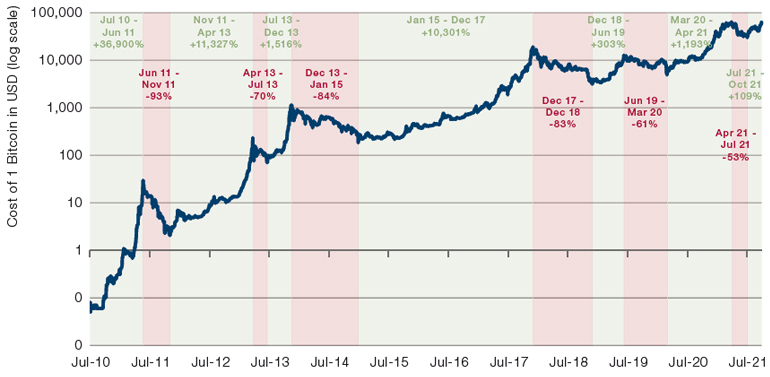
Source: Bloomberg. Bull and bear periods defined by the Man DNA team. As of 15 October 2021. The periods selected are exceptional and the results do not reflect typical performance. The start and end dates of such events are subjective and different sources may suggest different date ranges, leading to different performance figures.
Exhibit 2. Screenshot From ‘A Brief History of Bubbles’ (September 2018)
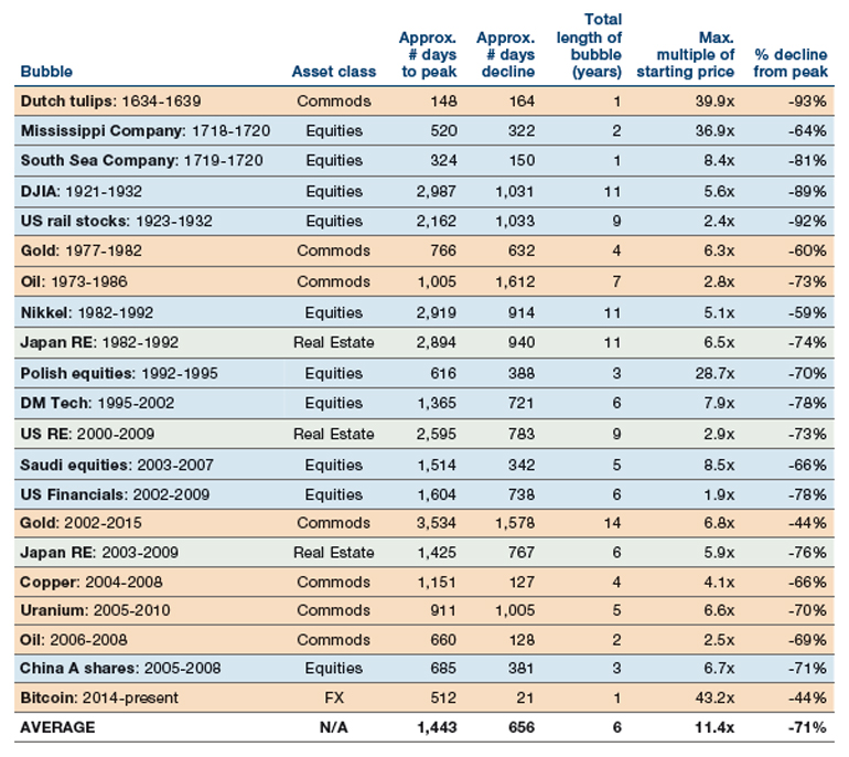
Source: Man DNA database.
Like Tyson Fury it takes some enormous hits, but repeatedly seems to fight back with a resurgence that stuns its detractors.
Bitcoin has followed a very different pattern, as Exhibit 1 attests. Like Tyson Fury it takes some enormous hits, but repeatedly seems to fight back with a resurgence that stuns its detractors.
The fact that it has done this so often in a short space of time is at least initial evidence that Bitcoin’s volatility is less bubble behaviour, and more the price discovery mechanism of a genuinely new asset class.
It may still be that the clothes come off the emperor. Indeed, it seems likely that, even if it endures, it has a few more 50% drawdowns left in it. But, given the above, we think the time has come to think seriously about it as a potential investment and, from our perspective, how it might fit into a multi-asset portfolio. This note represents a first attempt to put some numbers around our thoughts. We discuss Bitcoin and Crypto broadly synonymously, given that the former provides the best longterm proxy data for the latter, but also discuss some of the rationale for diversification within a Crypto sleeve.
What Is the Rationale for Crypto and How Should it Be Valued?
Various fundamental cases have been put forward for Bitcoin, and Crypto more generally. In its early days the libertarian argument of it being a new unit of exchange, whose use was shielded from the prying eyes of big government, was at the forefront. Increasingly, and especially since the monetary and fiscal largesse in the wake of Covid-19, the debate has shifted to whether the currency represents an investment free from the prying interventions of central bankers. Twenty-eight percent of all M2 dollars have been created in the last two years.1 These numbers have started to leak out of the dry domain of academic economists, into mainstream discourse. In that context the allure of an asset which features a hard stop at 21 million units, and cannot be printed at the whim of a policymaker or corporate board, is being more seriously and widely considered.
Like gold or art, Bitcoin has no yield and is not a currency in so far as you cannot pay your taxes in it. It therefore has no intrinsic value that would be recognised under a discounted cash flow (‘DCF’) framework. While that is a problem, we think that an asset doesn’t necessarily need to have DCF-oriented fundamental value to be useful in a whole-of-portfolio context. In a world where printing presses are whirring, as already alluded to, and a higher inflation regime, while not a certainty, is surely a bigger risk than it was two years ago, Bitcoin may, like gold, have value as a hedge against debasements of more conventional currencies.
One common pushback is the argument that central bankers, and Treasuries more broadly, are not going to allow themselves to be disintermediated. Given that they write the rules, they can simply regulate the ‘problem’ away. We think this is not at all inconceivable. But we would point out that, with a current capitalisation of $1.1trn, if Bitcoin was a stock it would already be the fifth biggest in the S&P 500 Index, in between Amazon ($1.8trn) and Tesla ($1.0trn).2 Clearly anything can be broken up, but it is also true that there is a size where it becomes harder for regulators to do so.
Assuming the regulatory hard stop does not transpire, we are still left with the question of how to value this novel asset without underlying cash flows. One method is to take the gold comparison already discussed, and assume that Bitcoin is on a trajectory to take some share of this currency-debasement-hedge pie.
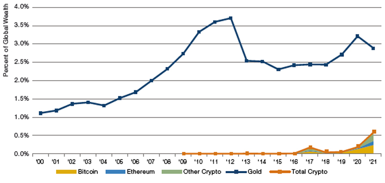
Exhibit 3 shows the total value of ‘above ground’ Gold and Crypto, as a percentage of total global wealth. At time of writing:
- We estimate the world’s wealth to be $446trn;
- We suppose that the total volume of Gold ever mined is 204k metric tonnes which, at current prices, is equal to $13trn or 3% of global wealth;
- Just short of 19m Bitcoin have so far been mined which is equal to $1.2trn or 0.3% of global wealth;
- Bitcoin makes up about half of all Crypto, with Ether a further 20%, and a long tail of some 8,000 other coins making up the remaining 30%.3
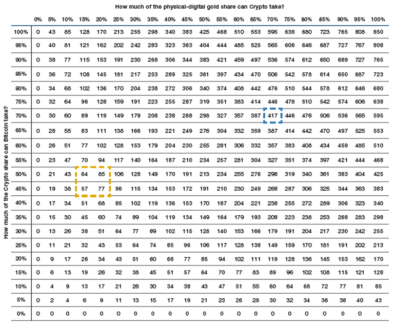
In a scenario where Crypto grew to 70% of physical-digital gold, and Bitcoin’s share of Crypto rose to 70%... the price could rise to $417k, or about 600% from current prices.
In other words, if the ‘digital Gold’ argument is right, then Crypto still has a long way to travel. Currently global Gold plus global Crypto is worth some $16trn, with the latter making up around 16% of this total. In Exhibit 4 we show various scenarios for the price of Bitcoin assuming movements in Crypto’s share of this physical-digital gold pie (on the x axis), as well as changes in Bitcoin’s share of the Crypto universe (y axis).
Currently we are in the area outlined in orange. In a scenario where Crypto grew to 70% of physical-digital gold, and Bitcoin’s share of Crypto rose to 70% (possibly off the back of consolidation in the long tail of other coins already described), then, as indicated in dashed blue, the price could rise to $417k, or about 600% from current prices. This is not a prediction, but it does demonstrate that there is a case to be made, apart from debates around underlying cash flows.
Clearly there is no guarantee that Bitcoin will retain its Crypto-crown. To counter the risk that, per Exhibit 4, Crypto goes to 70% of the physical-digital gold share, but Bitcoin goes to 0% of Crypto, it may make sense to have some diversification within any Crypto sleeve. In general the major tokens tend to move in similar fashion; for instance, the daily correlation between Bitcoin and Ethereum since the start of 2018 (where we have reliable data for the latter) is around 0.8.
Exhibit 3. Gold and Bitcoin as Percent of Global Wealth
Source: Credit Suisse, World Gold Council, Statista, Bloomberg, Man DNA team calculations. See footnote 3 for further detail.
Exhibit 4. Implied Price of Bitcoin (in USDk) under Different Scenarios
Source: Man DNA calculations.
Where Does Crypto Sit on an Initial Smell Test?
Exhibit 5 shows the basic building blocks of a multi-asset portfolio, divided into Equities, Fixed Income and Alternatives, the last of which being our initial repository for Crypto (which we proxy with Bitcoin). We also include long/short equity factors at the bottom of the table, given that they form an important part of our research. For each asset we show summary statistics for the period over which we have daily Bitcoin data.
Crypto has been a shoot-the-lights-out asset, not only on a simple return basis, but also on a risk adjusted reading.
From this we would make two initial observations. First, Crypto has been a shootthe-lights-out asset, not only on a simple return basis, but also on a risk-adjusted reading. Its Sharpe ratio of 2.3 is well over a point higher than its closest competitor, being High Yield Credit.
There can be a world of difference between a risk model which solves for volatility, and one that solves for drawdown, however. And our second observation is that the drawdown on Crypto has been far worse than other segments. At -81% it is over 2.5x the nearest rival, Commodities on -32%. So this is the wrinkle. The risk-adjusted return may be attractive but whether investors have the behavioural gumption to hold the line through the drawdowns, thereby achieving those numbers, is far from certain. These considerations drive our next two lines of interrogation.
Exhibit 5. Risk and Return Statistics, July 2010 to Present
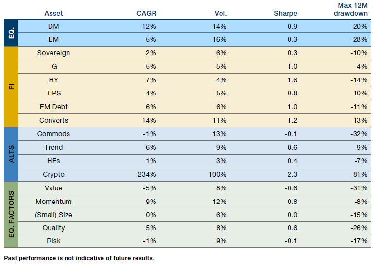
Source: Bloomberg, Man AHL, Goldman Sachs, Man DNA team calculations. Assets proxied as follows: DM Equity = MSCI World Local Currency, EM Equity = MSCI EM USD, Global Sovereigns = Bloomberg Barclays Global Agg Treasuries, IG = Bloomberg Barclays US IG Corporates, HY = Bloomberg Barclays US HY Corporates, TIPS = Bloomberg US Government Inflation Linked All Maturities, EM Debt = JP Morgan EMBI Global Composite, Converts = Bloomberg US Convertible Composite, Commods = Bloomberg Commodity Index TR, Trend = Man AHL global trend estimate, HFs = vol. scaled equal weight portfolio based on L/S equity portfolios for Value, Momentum, Size, Quality and Risk, across Europe and US. Indices constructed by Goldman Sachs. Crypto = Bitcoin against USD, factors are L/S equity indices from GS.
How Does Crypto Move in Relation to Other Assets?
In Exhibit 6 we show a pairwise correlation matrix for the same assets as were listed in Exhibit 5 (with the addition of Gold individually), circling Crypto’s numbers in blue. Generally, the asset class moves in a strongly differentiated pattern to the investable universe. Ignoring signs, the average pairwise correlation for Crypto is easily the lowest of our portfolio building blocks and, between friends, we’d call it zero. We illustrate this in Exhibit 7.
Exhibit 6. Correlation Matrix (2010 to Present) for Assets in Exhibit 5
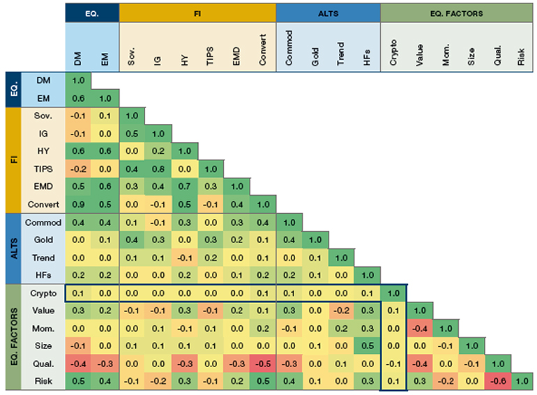
Source: All per Exhibit 5. Gold is TR on Gold futures from Bloomberg. Correlations calculated on daily periodicity by Man DNA team.
Exhibit 7. Average Pairwise Correlation (Ignoring Signs), Calculated off Exhibit 6
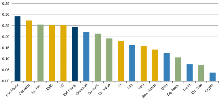
Source: Calculated by Man DNA team off data from Exhibit 6.
The average pairwise correlation for Crypto is easily the lowest of our portfolio building blocks and, between friends, we’d call it zero.
So for investors holding Crypto as part of a broader asset allocation there is surely an argument that its purpose in the portfolio is as much about diversification as it is about pure return. To take a sporting analogy, that it is as much a gritty holding midfielder, as it is a flair number 10. This can help add behavioural ballast, allowing positions not to wobble in the holes identified in the previous section.
How Does Crypto Move in Relation to Other Assets When Times Are Hard?
Correlation in general is far from the end of the story, of course. Left tail correlations are at the heart of our risk management process because our view is that the Black Monday / DotCom / GFC / Covid type sell-offs are the times when you most want promised diversification to kick in.
In Exhibit 8 we show the drawdowns and negative hit rates for the 344 instances since July 2010 where Crypto had sold off by 20% or more month-on-month. This is equal to 12% of the time. This gives us a first clue as to a worryingly risk-on relationship. Assets more closely associated with risk-on attitude tend to sell off more and with more consistency than those less so.
So Equity is negative on average, as is High Yield, EM Debt and Converts, all segments of the Fixed Income universe with higher equity betas. Similarly, Commodities, a clear global cyclical bellwether, as well as Value, Small Cap and Risk in Equity L/S space, tend to suffer coincident with Crypto.
Exhibit 8. Asset Performance where Crypto Falls 20% or More MoM (2010 to Present)
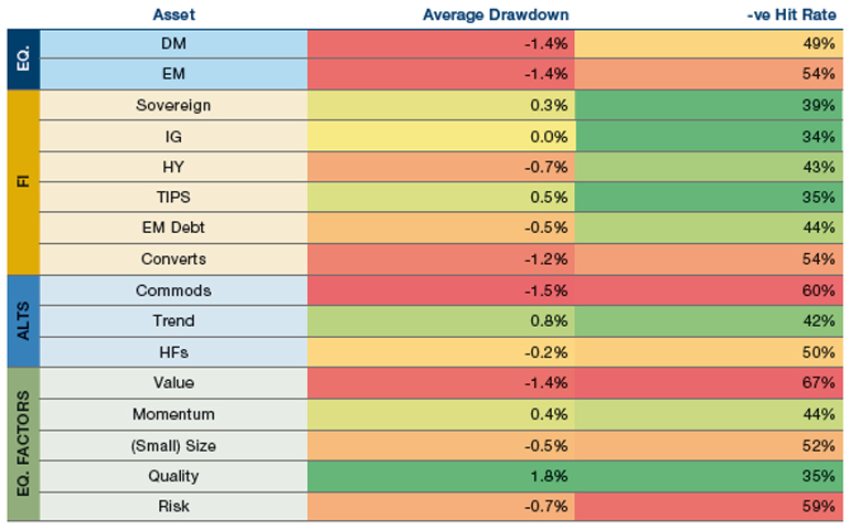
Source: See source note on Exhibit 5.
What will Crypto do for you when your traditional betas are leaving you bloodied and bruised in a ditch.
But a more practical way of looking at the problem is the other way around, what will Crypto do for you when your traditional betas are leaving you bloodied and bruised in a ditch. Within our timeframe we therefore look at how digital currencies have performed during 1-month drawdowns of 5% or more for Equity, and of 2.5% or more for 60/40. These thresholds cover 6% and 7% of our time sample respectively.
We first demonstrate our results graphically in Exhibit 9. Here we show the 17 occasions in which DM Equities have drawn down 5% or more over a short period of time (here we are defining the regimes more qualitatively). For each drawdown we show the daily cumulative total return to Equity (in blue) and Crypto (in yellow). We then decide whether in each instance Crypto was a good diversifying asset (green ‘+’), a bad one (red ‘X’) or neutral (grey ‘=’). Total scores are 9 ‘X’, 4 ‘=’ and 4 ‘+’. There might be a couple you could argue the toss on, but it doesn’t add up to much whichever way you cut it.
Exhibit 9. Equity Drawdowns since 2010 and How Crypto Performed
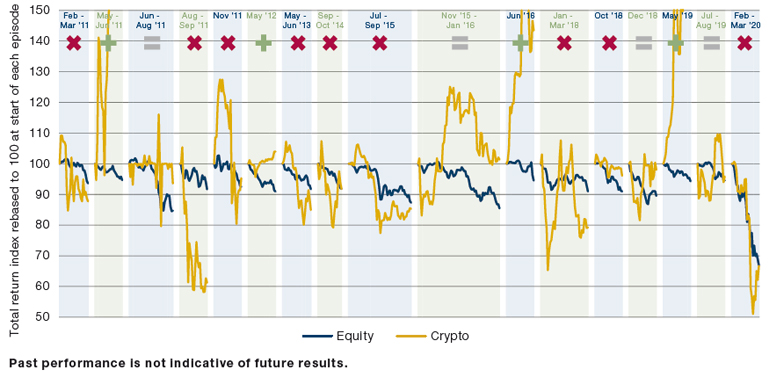
Source: Man DNA team. As of 15th October 2021. The periods selected are exceptional and the results do not reflect typical performance. The start and end dates of such events are subjective and different sources may suggest different date ranges, leading to different performance figures.
The same message is borne out under a more scientific approach. In the 6% of instances where the equity market sold off 5% or more over a one month period:
The co-movement between the digital currency and traditional market betas is three times greater in a correction environment than in general.
- The average performance of Bitcoin was -13%;
- Bitcoin registered a negative return 86% of the time;
- The left tail correlation was 0.3. Similarly, in the 7% of instances where 60/40 registered a 2.5% monthly drawdown:
- The average performance of Bitcoin was -10%;
- Bitcoin registered a negative return 79% of the time;
- The left tail correlation was 0.3.
Over the full time period, the correlation between Crypto and DM Equity is 0.1, per Exhibit 5. That between Crypto and 60/40 is also 0.1. So we can say that the comovement between the digital currency and traditional market betas is three times greater in a correction environment than in general. Clearly, this is not a promising quality
Given All of This What, if Any, Is the Right Crypto Allocation?
Thus far we have observed that Crypto is:
- An attractive asset when viewed on a traditional return per unit of risk basis;
- An unattractive asset when looked at through the prism of drawdowns;
- An attractive asset in that it provides high levels of diversification in general, but…
- …an unattractive asset in that its diversification benefit shrinks markedly in a traditional market beta sell-off.
The question remains as to how these variables should be weighted, so as to answer the question of what an appropriate allocation looks like. As a first cut at answering this we take a generalised reduced gradient optimisation approach, to construct two example portfolios, one with Crypto and one without. We use the following parameters:
- We assume 12 books being those illustrated under ‘EQ’, ‘FI’ and ‘ALTS’ in Exhibit 5;
- Each book must have an allocation of at least 2%;
- The total Equity allocation must be between 15% and 45%;
- The total Fixed Income allocation must be between 30% and 90%;
- The total Alternatives allocation must be between 30% and 50%;
- The maximum drawdown over any one month must not exceed 15%;
- Solve for maximum Sharpe.
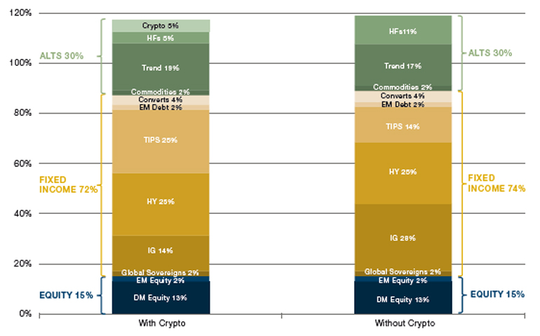
This analysis yields the two portfolios shown in Exhibit 10. From this we observe that the With Crypto portfolio relative to the ‘Without’ is:
- Marginally more capital efficient (total exposure of 117% vs 119%);
- Significantly under exposed to Hedge Funds (equity long / short strategies);
- Marginally over exposed to Trend;
- Marginally under exposed to Fixed Income;
- Significantly over exposed to TIPS;
- Significantly under exposed to IG.
Exhibit 10. Sharpe Optimised Portfolio Allocations With and Without a Crypto Component
Source: Man DNA team. Example for illustrative purposes only. Hypothetical results are calculated in hindsight, invariably show positive rates of return, and are subject to various modelling assumptions, statistical variances and interpretational differences. No representation is made as to the reasonableness or accuracy of the calculations. Since trades have not actually been executed, hypothetical results may have under or over compensated for the impact, if any, of certain market factors.
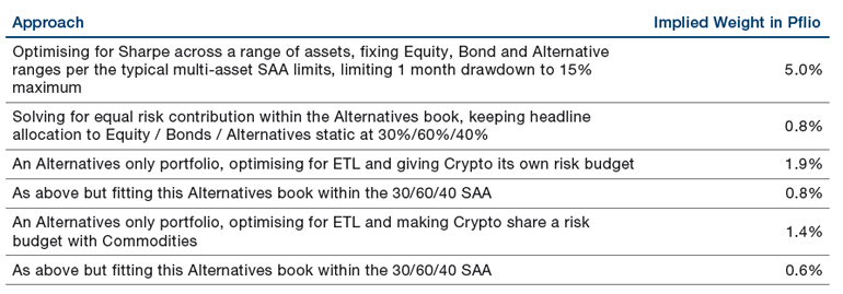
Exhibit 11 shows how these two allocations would have performed, along with some summary statistics. We think this illustrates the trade-off that asset allocators face: on the one hand Crypto-inclusion is a significant positive for Sharpe, adding 0.7 points. But that is paid for with a worse drawdown profile, both in terms of their happening with greater regularity (38 5% drawdowns vs 26), and greater severity (as illustrated in the pink shaded areas). Whether that trade-off is worthwhile is ultimately a subjective choice. But for those wanting to swallow the medicine, an allocation of around 5% could make sense, based on this analysis.
A different optimisation approach is to solve for an equal risk contribution within the Alternatives sub-books, rather than a risk-adjusted return at the portfolio level. This would entail the following:
- Keep weights of Equity, Fixed Income and Alternatives static at 30 / 60 / 40% (a common multi-asset SAA in our experience);
- Within Equity and Fixed Income keep the weights of all sub-books constant at SAA weights (30% DM Equity, 53% DM Sovereigns and 7% EM Debt);
- With Alternatives make the risk contribution of each of the sub-books equal.
Following this approach, we get a much lower weighting to Crypto, at 0.8%. In the bottom panel of Exhibit 11 we chart the performance of ‘With’ and ‘Without’ on this updated methodology. The difference between the two portfolios is now much narrower in risk-adjusted return space, but also in terms of frequency of drawdown, with the inclusive portfolio experiencing just two additional corrections (24 vs 22).
In our portfolio construction work we have often used a clustered inverse expected tail loss (‘ETL’) approach. This keeps allocations within the 30% Equity and 60% Bond portions static (weights according to the typical multi-asset SAA, as discussed above), but within the 40% Alternatives book, weights the individual sleeves optimising for ETL, but with the different allocations clustered according to common risk budgets. So, for instance, we group Momentum and Seasonality given that they share a Trend factor risk component. If we follow this methodology giving Crypto (proxied by Bitcoin) its own risk cluster we get an optimal weight of 1.9% of the Alternatives book, or 0.8% if within the full 30/60/40 example portfolio SAA. If we do the same but make Crypto share a risk budget with Commodities (by merit of the inflation hedge argument already discussed), we get equivalent numbers of 1.4% and 0.6%.4
In Exhibit 12, we show a summary table with all the different optimisation approaches we have considered.
Exhibit 11. Performance of Portfolios Illustrated in Exhibit 10 (Top) and Using Alternate Optimisation Parameters (Bottom)
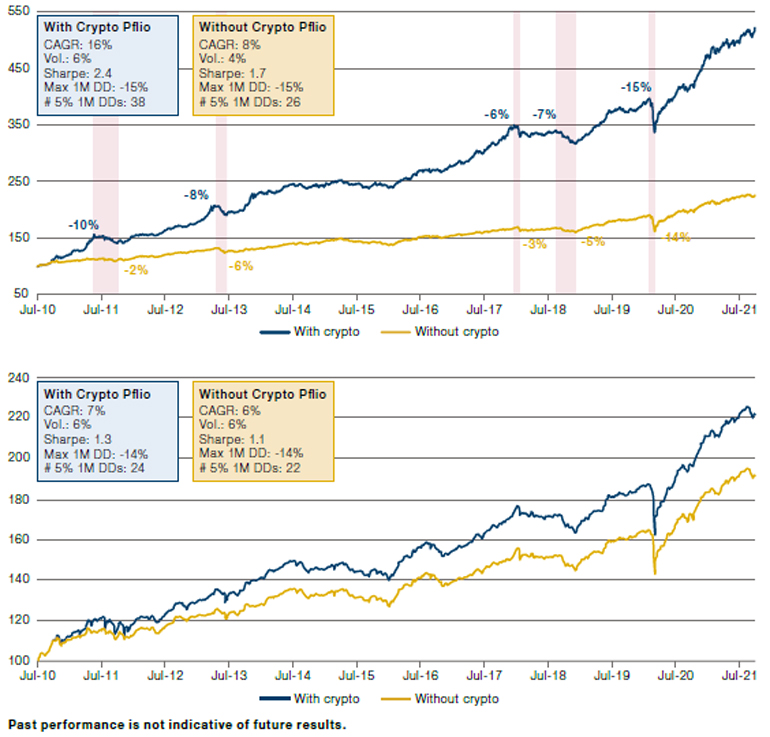
Hypothetical results are calculated in hindsight, invariably show positive rates of return, and are subject to various modelling assumptions, statistical variances and interpretational differences. No representation is made as to the reasonableness or accuracy of the calculations. Since trades have not actually been executed, hypothetical results may have under or over compensated for the impact, if any, of certain market factors.
Exhibit 12. Summary Table of Crypto Optimisation Approaches
Source: Illustrative example – for information only. The above example is intended as an illustration of typical investment considerations and strategy implementation. It should not be construed as indicative of potential performance of a fund or strategy or of any investment made by a fund or strategy. The above are indicative targets, restrictions, attributions, constituents and limits which are provided for illustrative purposes only. Underlying vehicles may have their own distinct mandate restrictions
Practical Considerations
Crypto also presents a number of issues not directly related to investment performance. We will touch on a couple of these very briefly here, as a placemarker for further work. One is implementation. A UCITS vehicle cannot invest in crypto-coins in ‘physical’ (irony intended) or derivative format because they are currently not deemed to be ‘transferable securities’ in accordance with the UCITS definition. Given that Crypto ETFs launched thus far are not UCITS equivalent, this route is also unavailable at present. Because ETNs are generally seen as debt, rather than equity instruments, there is potential for their use to allow UCITS schemes to gain exposure, however this path has not been widely tested from a legal perspective, and it is likely that internal compliance departments will be somewhat nervous around it.
A further concern is the ESG angle. Various papers estimating the energy intensity of mining and transacting in Bitcoin have put the total as equivalent to various countries, such as Argentina and New Zealand. In short, a lot. To give some context it is estimated that every Bitcoin transaction consumes 1,173 kilowatt hours of electricity, about what the typical American home will use in 6 weeks.5
There are a couple of nuances to this; Ethereum’s Altair upgrade, which went live in October this year, should ultimately reduce the token’s energy usage by 99%, by moving from a proof-of-work to a proof-of-stake model. A further argument, perhaps, for diversification between tokens within a Crypto allocation. In addition, China’s crackdown on Bitcoin through the summer pushed significant activity over to America. This is a likely driver behind a dramatic halving in its energy usage from around 140 terawatt hours a year, to ‘only’ 70, as more inefficient mining capacity was taken offline.6 This is still a huge total (0.33% of the world’s energy production) but does illustrate the potential for enhancements in this area.
1. Per Bloomberg data. Henceforward, unless otherwise stated, all data sources are Bloomberg.
2. As at 18/11/2021. Source: Bloomberg. The organisations and/or financial instruments mentioned are for reference purposes only. The content of this material should not be construed as a recommendation for their purchase or sale.
3. Sources: Global wealth statistics from Credit Suisse, gold statistics from the World Gold Council, coin mining statistics from Statista, while all prices from Bloomberg.
4. We are heavily indebted to the work of Davide Malizia on the Man FRM quantitative portfolio construction team for assisting us in the clustered ETL analysis.
5. Per a study from Money Super Market: https://www.moneysupermarket.com/gas-and-electricity/features/crypto-energy-consumption/
6. As reported by CNBC: https://www.cnbc.com/2021/07/20/bitcoin-mining-environmental-impact-new-study.html
Hypothetical Results
Hypothetical Results are calculated in hindsight, invariably show positive rates of return, and are subject to various modelling assumptions, statistical variances and interpretational differences. No representation is made as to the reasonableness or accuracy of the calculations or assumptions made or that all assumptions used in achieving the results have been utilized equally or appropriately, or that other assumptions should not have been used or would have been more accurate or representative. Changes in the assumptions would have a material impact on the Hypothetical Results and other statistical information based on the Hypothetical Results.
The Hypothetical Results have other inherent limitations, some of which are described below. They do not involve financial risk or reflect actual trading by an Investment Product, and therefore do not reflect the impact that economic and market factors, including concentration, lack of liquidity or market disruptions, regulatory (including tax) and other conditions then in existence may have on investment decisions for an Investment Product. In addition, the ability to withstand losses or to adhere to a particular trading program in spite of trading losses are material points which can also adversely affect actual trading results. Since trades have not actually been executed, Hypothetical Results may have under or over compensated for the impact, if any, of certain market factors. There are frequently sharp differences between the Hypothetical Results and the actual results of an Investment Product. No assurance can be given that market, economic or other factors may not cause the Investment Manager to make modifications to the strategies over time. There also may be a material difference between the amount of an Investment Product’s assets at any time and the amount of the assets assumed in the Hypothetical Results, which difference may have an impact on the management of an Investment Product. Hypothetical Results should not be relied on, and the results presented in no way reflect skill of the investment manager. A decision to invest in an Investment Product should not be based on the Hypothetical Results.
No representation is made that an Investment Product’s performance would have been the same as the Hypothetical Results had an Investment Product been in existence during such time or that such investment strategy will be maintained substantially the same in the future; the Investment Manager may choose to implement changes to the strategies, make different investments or have an Investment Product invest in other investments not reflected in the Hypothetical Results or vice versa. To the extent there are any material differences between the Investment Manager’s management of an Investment Product and the investment strategy as reflected in the Hypothetical Results, the Hypothetical Results will no longer be as representative, and their illustration value will decrease substantially. No representation is made that an Investment Product will or is likely to achieve its objectives or results comparable to those shown, including the Hypothetical Results, or will make any profit or will be able to avoid incurring substantial losses. Past performance is not indicative of future results and simulated results in no way reflect upon the manager’s skill or ability.

You are now leaving Man Group’s website
You are leaving Man Group’s website and entering a third-party website that is not controlled, maintained, or monitored by Man Group. Man Group is not responsible for the content or availability of the third-party website. By leaving Man Group’s website, you will be subject to the third-party website’s terms, policies and/or notices, including those related to privacy and security, as applicable.