Capital Market Assumptions: Redefined

Introduction

CMAs seek to help allocators with their asset allocation decisions by establishing long-term forecasts for different financial assets. The problem is that they either fail to do this with much accuracy or make their forecasts with such a degree of caution that the output is of limited practical use.

In this paper, we propose a framework to help allocators to calculate these assumptions for themselves, as well as explore some practical applications for the resulting data.

A critical question that is not given sufficient consideration in our view is: what are you proposing to use CMAs for? There seem to be two options. First, allocators may have a liability window over the next 10 years, and want a base case for how assets might match these liabilities. Or secondly, they may want an unconditional base rate which serves as the foundation for ultra-long portfolio allocations. If the latter, and we suspect this is the case for most users, then the timeframe consideration becomes particularly important.

In Part One, we discuss forecast timeframes. In Part Two, we describe four credible methods for determining CMAs. In Part Three, we use findings from the prior two sections to calculate a range of CMAs for US stocks and 10-year Treasuries (UST10). These assumptions allow us, in Part Four, to derive strategic asset allocations (SAA), based on optimisation parameters such as return, volatility drawdown and Sharpe ratio.

In this paper we focus only on US equities and intermediate duration, as the two most consequential portfolio building blocks.

Part One: CMA timeframes

Inherent in CMAs is the idea that asset returns are more predictable on a long-term horizon than on a short-term view. In Figure 1, we show the distribution of one- and 10-year rolling returns to US stocks and bonds, over the ultra-long-term.

Figure 1. Distribution of returns for US stocks (top) and bonds (bottom), 1800-2024

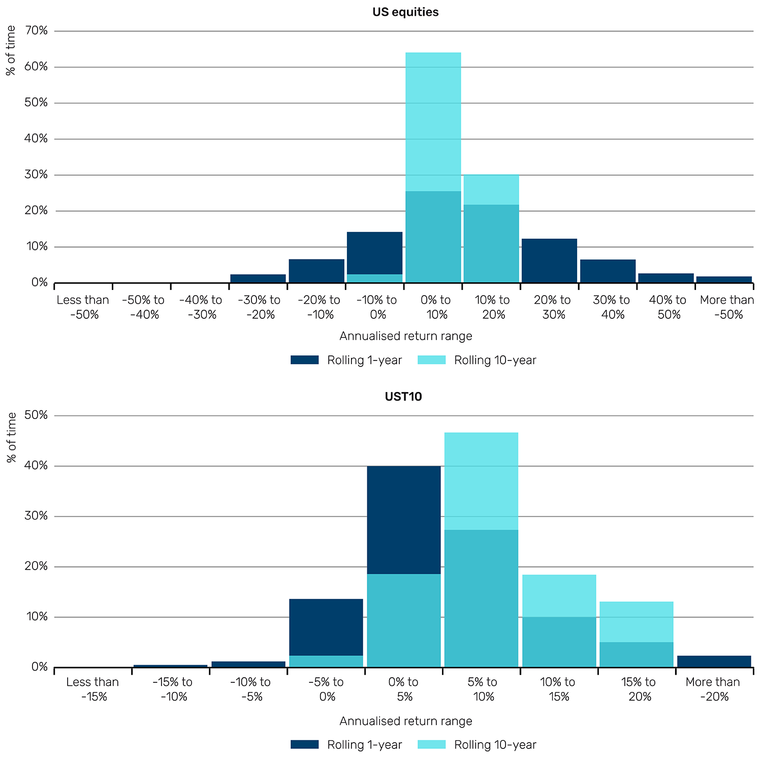
Source: GFD, Man Group. As of December 2024.

For stocks, the distribution becomes dramatically compressed as the return lookback is increased. On a 10-year annualised basis, 93% of returns fall into the 0-20% annual return buckets (on a one-year basis, the figure is 49%). However, the 10-year range is still wider than might be expected. There are 547 instances where returns were either below 4% annualised, or above 16% annualised, collectively accounting for over a fifth of history. Imagine that you’re a US$100 billion endowment or sovereign wealth fund advising your stakeholders on the kind of distributions they can expect based on long-term forecasts. These two pathways diverge by almost US$300 billion.

From Figure 1, we can also see that the distribution compresses more for equities than for bonds as the return window rises. For bonds, the 0-10% bands represent 68% of rolling one-year observations, and 66% of rolling 10-year periods.¹

Most investors’ instinctive outlook duration is 10 years. But it is debatable whether this represents an unconditional base rate, at least considering historic precedent. In the case of equities, your forecast horizon might need to be longer than you think, and applying the same timeframe for all assets could risk oversimplification.

Part Two: CMA methodologies

With these limitations in mind, we now offer four credible methods for determining CMAs.

The simple historic method

The simple historic method looks at returns over the very long term, i.e., it is an aggregation of as much historic data as is attainable for the given asset. For US stocks, this has been 8.7% (1800 to 2024). For US bonds, this has been 5.0% over the same period.²

While this is a potentially attractive route to establishing an unconditional base rate, we would repeat the warning from Part One – the next 225 years could be very different to the last. To illustrate, consider that equities can be seen as a levered play on nominal GDP. The rate of nominal GDP growth in developed economies over long windows has been highly variable. In Figure 2, we show 225-year annualised nominal GDP growth for the UK for four discrete windows since 1270 (calculated from the Bank of England’s Millenium of Macroeconomic Data resource).

By all means, take an ultra-long history as a base rate to inform future expectations. But remember to hold it lightly.

Figure 2. UK annualised nominal GDP growth split into 225-year discrete windows

Problems loading this infographic? - Please click here

Source: Bank of England, Man Group. As of February 2025.

The conditional historic method

The conditional historic method takes the same historic data, but conditions it based on starting valuation. It employs the apparent truism that a higher starting valuation should result in a lower forward return. If we take the smoothed earnings yield on equities as a proxy for return, and the same for the yield-to-maturity on US Treasuries, we see an attractive fit between starting valuation and forward return, at least on an overlapping basis (Figure 3).

Figure 3. Relationship between starting valuation and 10-year forward return for US stocks (top) and bonds (bottom), 1881-2024

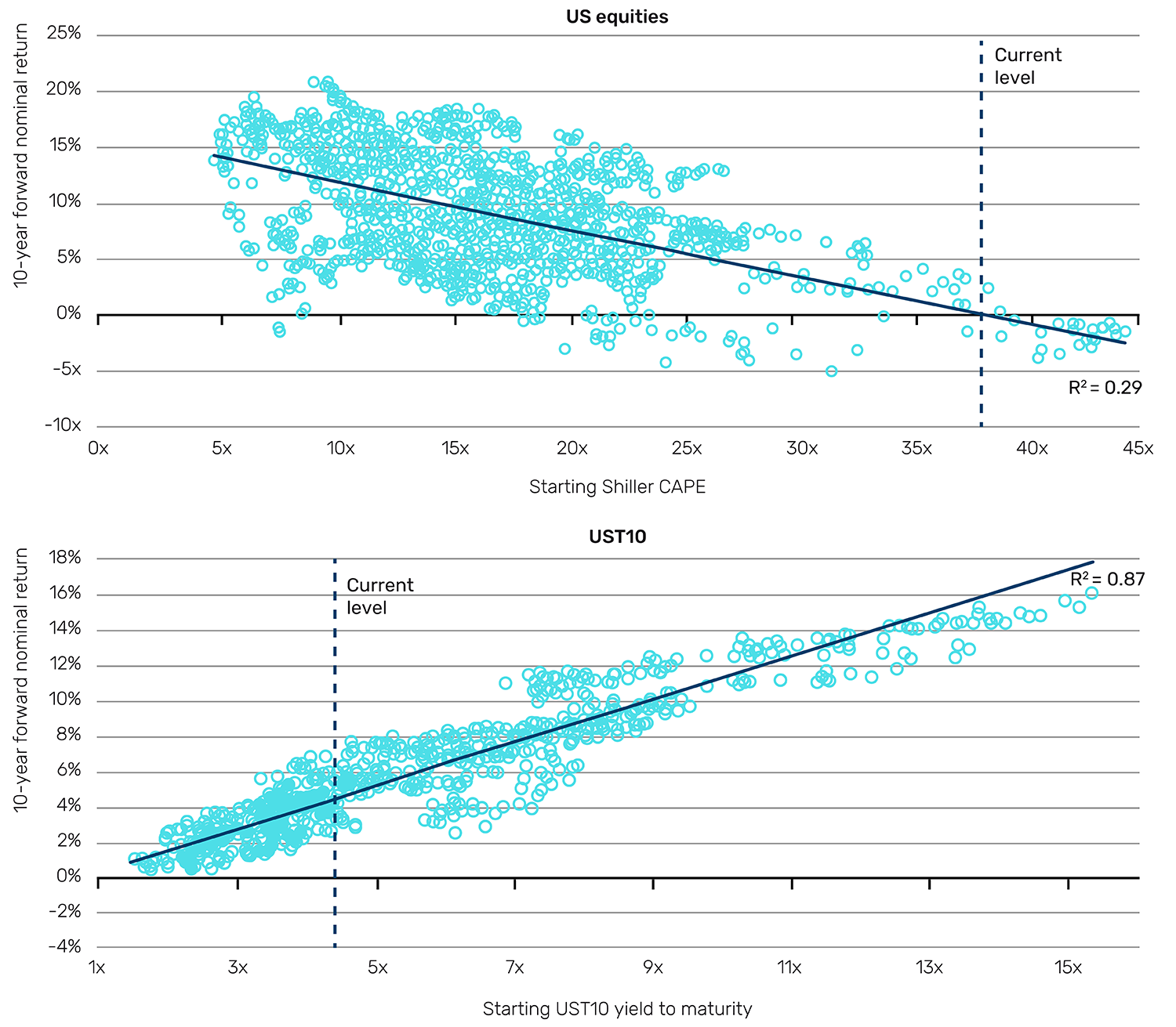
Source: Professor Shiller’s online database, GFD, Man Group calculations. As of December 2024.

If the historic precedent were to hold, we should expect 10-year nominal CAGRs³ to US stocks and bonds of 0% and 4%, respectively. Over the 150 years for which we have US inflation data, the lowest 10-year rolling inflation has been -4%, the average is +2% and the highest is +9%. Thus, for stocks, one could credibly forecast a range of real annualised returns over the next decade of between -9% and +4%, with a point estimate of -2%. This is bad news.

Arguably, these charts are melodramatic, given they use overlapping returns. So, while we think it a worthwhile exercise, we caution that it is easy to present such models in ways which are deceptively explanatory.

The theoretical method

The theoretical method involves building implied returns up from component parts based on current fundamental views.

The theoretical method applied to bonds

Given its importance, we start with the UST10 yield (which, as a by-product, will also give us an expected return for UST10).

We think about yield disaggregation as a three-part segmentation: trend growth, inflation expectation and term premium. When you lend money to the US government, or indeed any government with the ability to print the currency the bond is denominated in, you require compensation for these three things.

Constructing models that capture the essence of these three components is a huge undertaking and well beyond the scope of this paper. Moreover, there are already numerous indicators available for each.

In Figure 4, we show the range of a nominal set of indicators,⁴ as at the end of January 2025, along with their sum (fair value yield). After winsorising, this ranges from 3.6% to 7.4%, with a median of 5.5%.

Figure 4. Ranges of UST10 fair value yield using a selection of indicators

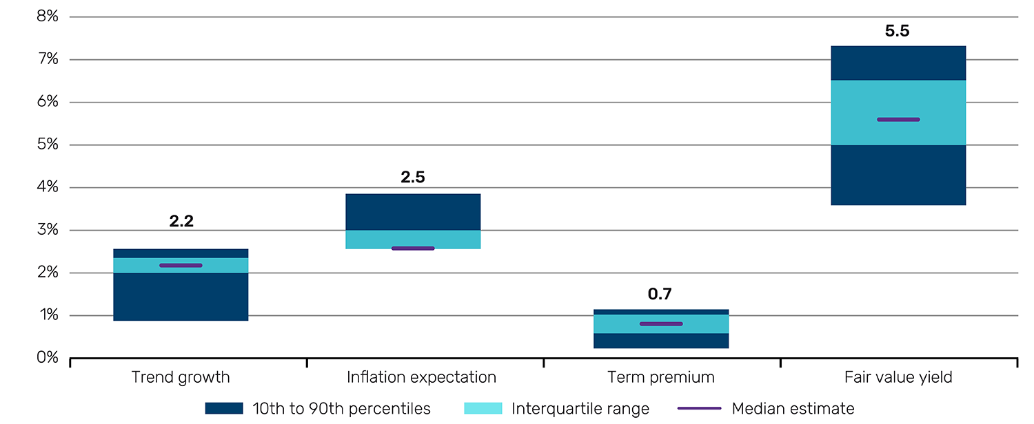
Source: Various sources as outlined in footnote 5, below. Collated from Bloomberg, NY Fed and the Livingston Survey. Levels calculated by Man Group. As of February 2025.

As at the end of January 2025, the yield and duration of the UST10 were 4.5% and 7.8%, respectively. Computing total return on a fixed income position is complex as it is influenced as much by the pathway of how interest rates change, as it is by the overall magnitude of the change. However, on a very simple basis⁵ this would translate into annual returns of +3.4% at the low end, and +4.7% at the top of the range, with a point estimate based on the median fair value yield of +4.2%.

The theoretical method applied to equities

The theoretical method also allows us to draw a baseline upon which to build a similar framework for equities. Because companies can (and do) raise debt, an equity can be viewed as a levered expression of aggregate economic growth. We have already accounted for trend growth in our decomposition of the bond yield. To determine the equity risk premium, or the increment over the Treasury curve that equity holders should theoretically demand, we need to account for changes in the overall risk profile of the economic backdrop.

One way of doing this is to find long-history metrics which gauge overall stress within an economy. This time, we have chosen six long-term measures of US economic risk.⁶ If these indicators are higher, potential turbulence is higher, and thereby the equity risk premium (ERP) should be higher to compensate.

In Figure 5, we combine these indicators and plot the aggregate alongside the Shiller excess CAPE yield.⁷ The higher the lines, the higher the implied economic risk, and the higher the ERP should be. Since the Global Financial Crisis (GFC), this metric has been relatively high, averaging 45%, bounded between 30% and 60%. That average would equate to an ERP of 7.5%. Currently, we are at the low end of the range, implying a premium of just under 4%. Both numbers are much higher than the current ERP of 1.1%. In other words, we’re looking at a significantly lower equity CAGR over the next 10 years than has been achieved over the last.

Figure 5. Aggregate economic risk indicator and Shiller excess CAPE yield

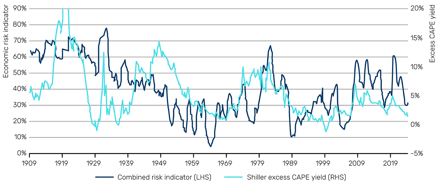
Source: Man Group calculations. As of December 2024.

To help give some quantum of how much lower, we can estimate nominal equity return on a 10-year forward view, implied by different UST10 yield levels combined with a range of ERPs. Unfortunately, our scenario analysis work implies an equity CMA in the 0 to -3% range, the most pessimistic estimate yet.

Meta-analysis

Another approach to CMAs is to simply take the average of everyone else’s estimates. We show the results of doing this for US equities and UST10 in Figure 6.

Figure 6. Third-party CMAs for US equities and UST10

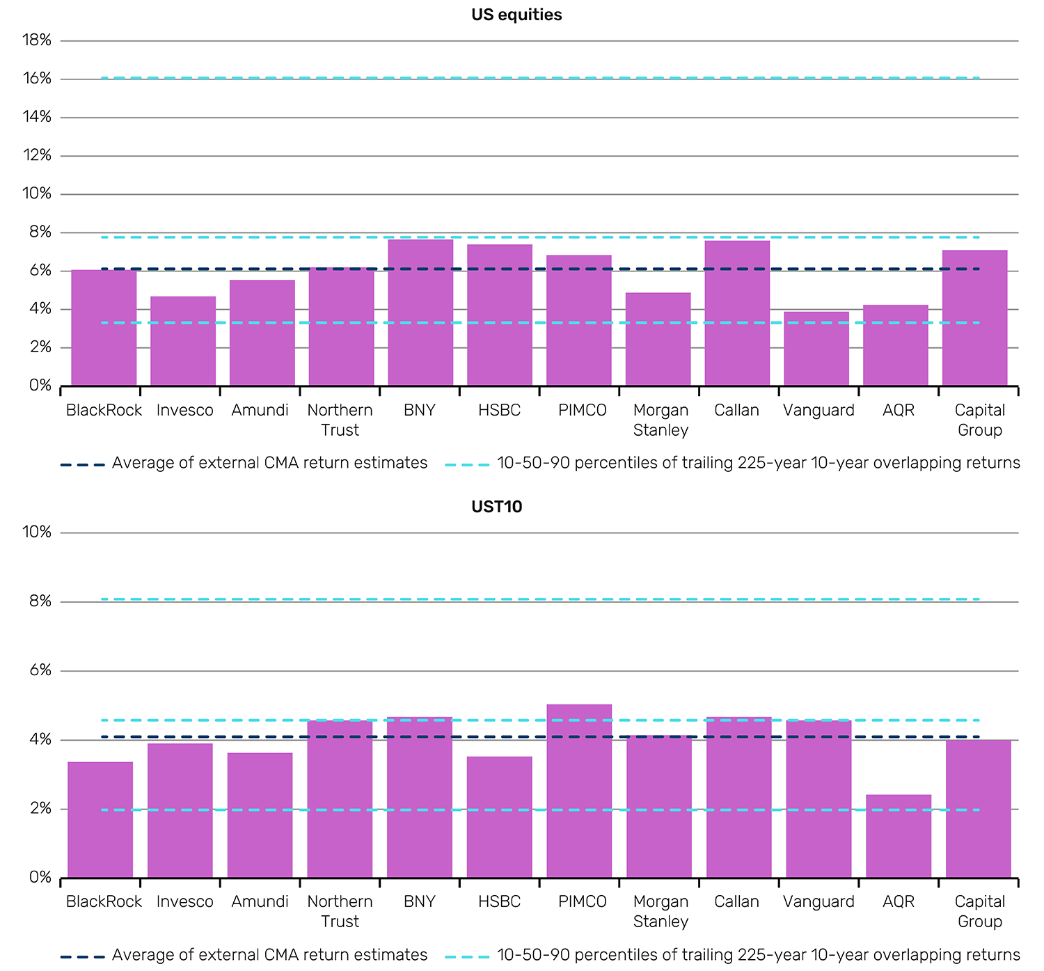
Source: Various asset manager websites, as indicated in chart. As of February 2025.

We note two things.

Firstly, consensus is relatively pessimistic on both equities and bonds. The navy blue dashed line shows the average estimate, while the aqua blue dashed lines show 10th-90th percentile range from Figure 1. We see the mean forecast is notably below the long-run historic median realised. For US equities, not one house meets this historic average level and for UST10, just five out of 12 do so. To that extent, they are within the context of that which we have seen so far: returns to beta over the next 10 years are likely to be inferior to those experienced over the last 10.

Secondly, within this relative pessimism, it is notable that no-one is reflecting the 0 to -3% equity rates that might be drawn from a valuation or economic fundamentals approach.

Part Three: CMA ranges for US equities and UST10

Return ranges

In Figure 7, we show a range of CMA returns for US equities and UST10, based on the various approaches we have described. As expected, the dispersion of equity projections is much greater (a range of 15 percentage points, compared with less than four for bonds), but the similarity in the medians is striking. For context, over the last 10 years, the gap between the two asset classes has been 12 percentage points (+13% for equities, +1% for bonds). Below suggests that, looking back a decade in 2035, we should not be staggered to see that spread having compressed to zero.

Figure 7. CMA return range based on methods previously outlined

Problems loading this infographic? - Please click here

Problems loading this infographic? - Please click here

Source: Compiled by Man Group using methods outlined in Part Two, as of February 2025.

For many users of CMAs, the story stops here. We note, however, that for the practitioner who needs to turn this into a practical SAA, this information, without corresponding volatility, correlation and drawdown assumptions, is of limited use.

Part Four: CMA implied portfolio combinations

To establish a base rate of how the differing combinations of equity and bonds have behaved, we can blend equity and bond portfolios with equity/bond proportions falling/rising in increments of 20 percentage points, alongside a simple risk parity portfolio.⁸ Again, we flag the critical importance of assumptions for volatility, correlation and drawdowns.

As expected, the higher bond-weighted portfolios are superior on a risk-adjusted basis, but inferior when viewed through an intrinsic return lens. For brevity, we can zone in on risk parity and the 60/40 portfolio (Figure 8).⁹

Figure 8. Summary statistics of 60/40 and risk parity portfolio combinations (1802-2024)

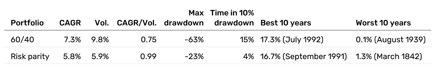
Source: Man Group calculations. As of December 2024.

It is hard to argue against risk parity, in terms of return, volatility, maximum drawdown and drawdown persistence. Less obviously, it is notable how good even 60/40 is as a combination: it is the highest equity-weight permutation never to be negative (at least in nominal terms) on a 10-year rolling basis.

In Figure 9, we show trailing return per unit of risk for the 60/40 and risk parity combinations, overlaid with bull-base-bear cases for the next 10 years (the dashed horizontal lines). Which assumptions one takes for return/risk/correlation, while based on Figures 7 and 8, are to some extent subjective. In the note below the chart, we outline the numbers we have used.

Figure 9. Return per unit of risk for 60/40 and risk parity, 1812 to 2024, with CMA portfolio projections

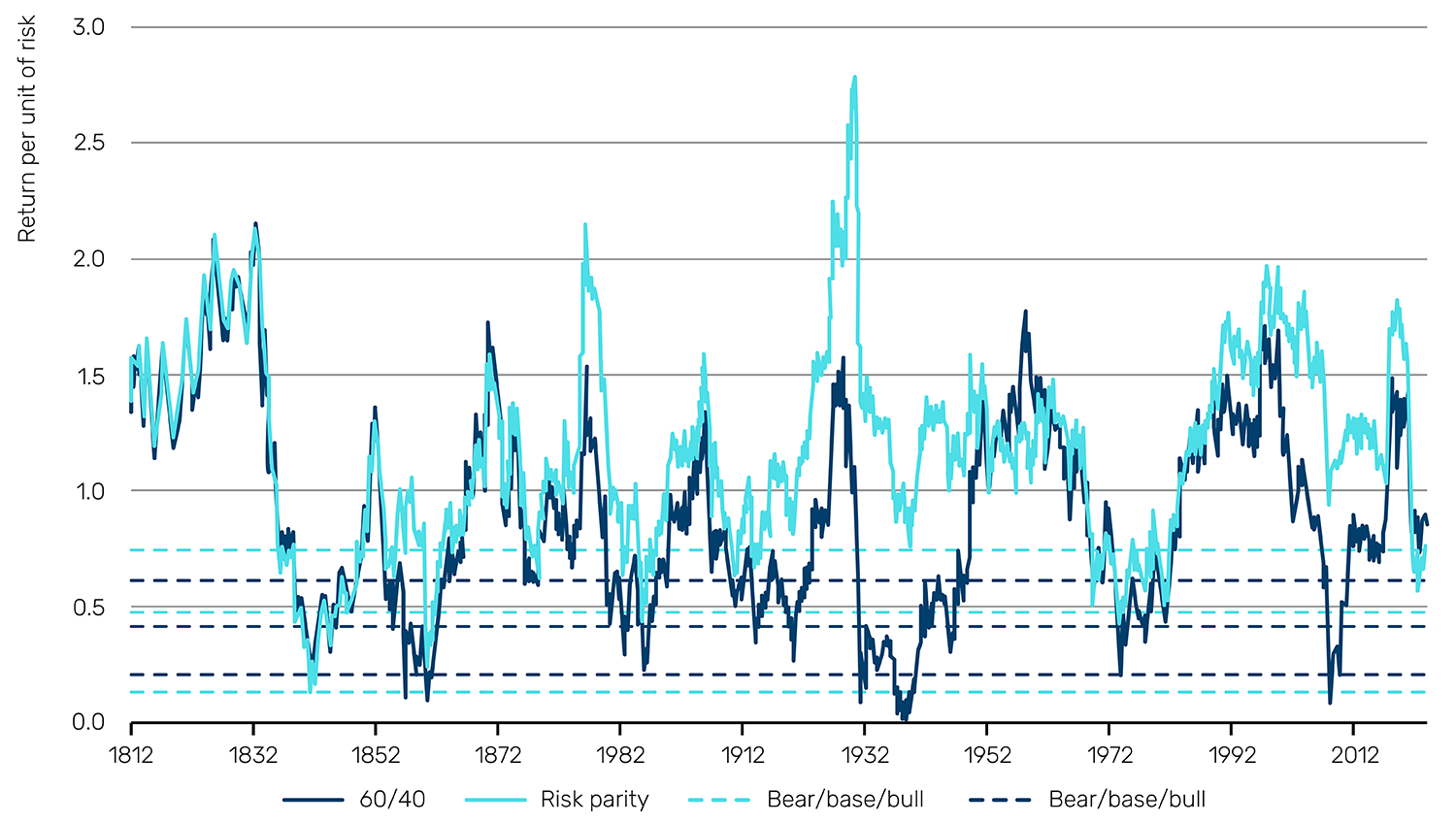
Source: Man Group calculations. As of December 2024.

Bear case assumes: CAGR: equity = +0.5%, bond = +3.0%, Vol.: equity = 17%, bond = 5.4%, Correl = +0.33. Base: CAGR: equity = +5.8%, bond = +4.1%, Vol: equity = 17%, bond = 4.1%, Correl. = +0.20. Bull: CAGR: equity = +7.5%, bond = +4.6%, Vol.: equity = 14.7%, bond = 4.1%, Correl. = -0.26.

Some observations.

First, apart from in extreme scenarios, it is likely that risk parity will again outperform 60/40 on a risk-adjusted basis through the next decade, as it has 81% of the time historically. Bearish pathways are the only exception.

Secondly, it may make sense to have a greater structural bond weight in your SAA than you would have opted for in 2015. The 10-year trailing UST10 return has almost never been lower and rarely stays in these doldrums for long. Per Figure 7, the CMA methodologies would suggest that the spread of equity to bond return going forward will be low compared to the past. Moreover, even in a positive stock-bond correlation world, Treasuries can still provide drawdown smoothing in left-tail equity events.¹⁰

The third lesson from Figure 9 is that, in the absolute sense, asset allocators should prepare to be disappointed, at least relative to recent experience, whichever SAA they opt for. Base cases for both portfolios over the next 10 years are meaningfully lower in the risk-adjusted space compared with the last 10 years.

Strategic mitigants for lower return environments

If this is to be a drier period for core portfolio allocations, what mitigants might we adopt?

The first is leverage. If equity and bond premia have excess returns, then its judicious use can help bring dollar returns to a sufficient level to meet their attached liabilities. One problem is that, as leverage increases, the potential for unforeseen issues is also elevated (the LDI crisis of September 2022 again comes to mind). Thus, hand-in-hand with leverage must come the deployment of a best-in-class risk overlay infrastructure.

The second potential solution is alpha. Alpha, however, can easily be swallowed up by costs, and it relies on skilful manager selection, as well as the continued skill of the manager themselves.

Thirdly, we suggest a more intense diversification of asset classes, outside of simple duration and equity beta. We see eight contenders¹¹ with the potential to meaningfully add value on top of equity and bond returns. The challenges here are twofold. First, many of these components are very speculative. And secondly, the more varied of these asset classes often have a high alpha component (positive or negative) – see above. From a CMA perspective, such an expansion often presents the challenge of data availability.

Another source of diversification is to stay within the lane of conventional public equity and sovereigns, but to vary geography beyond the US. Unfortunately, over long timeframes, there is typically a relatively high correlation, even between developed markets and emerging markets, assuming proper sub-security diversification. In some instances, however, and where valuation spreads between countries are high (as they are presently), the shape of theoretical forward returns can look quite different. Coming back to our CMA, while the methods described can certainly be applied to other geographies, data availability outside of the US is almost always inferior. Also, this path introduces the complexity of forcing you to take a CMA view on currency.

A final potential solution is greater cost consciousness. If it is the case that portfolio returns are going to be more modest than in the recent past, one option instead of reaching for return is to moderate spending. In other words, for the boards of asset owners to make peace with a more modest distribution profile for the next 10 years. This brings us to a pivotal issue for long term financial planning which we have hardly touched on: inflation. A general acceleration in price rises could undo an approach of frugality on its own.

Concluding remarks

Over the course of this paper, we have attempted to build a series of frameworks to help investors think about the purpose of long-term forecasting when it comes to portfolio construction. We have also highlighted the events or structural changes that could destabilise assumptions, as well as what could cause radical shifts in the distribution of returns or the concentration of risk. It is essential to question the underlying drivers of returns, and to analyse the assumptions that underpin these market forecasts, before seeking to employ them. We haven’t solved all the challenges of CMAs here, but we hope we have given the reader much to think about, and that you will approach these components of the asset allocation process with more healthy scepticism in the future.¹²

1. This makes sense as equity returns exhibit less autocorrelation than fixed income. Near-term bond returns have greater visibility of return due to higher cashflow predictability, so the aggregation benefit, in terms of reducing the return range, is less.
2. Past performance is not indicative of future results.
3. Compound annual growth rate.
4. We have used a wide variety of indicators for building UST10 components (approximately 20 across the three segments). If you would like to know the indicators used, please do get in touch.
5. Change in yield * duration + average of starting and ending carry, and assuming a 10-year horizon.
6. Percentage last 10 years in recession; percentage last 10 years in 10% drawdown; real GDP vol; inflation vol; BAA credit spread (12-month moving average [12MMA]); S&P vol (12MMA).
7. The purest way to calculate the equity risk premium is to compare the Treasury yield to the forward (i.e., expected) equity earnings yield. The Shiller excess CAPE yield is a decent proxy, based on the assumption that earnings expectation over the next 10 years, will be about the same as the last 10 years, adjusted for inflation.
8. Defined on a three-year lookback and with no leverage (i.e., weights always sum to 100%).
9. Again, if you would like to see the full summary statistics of different portfolio combinations between 1802-2024, please get in touch.
10. The 2021-22 experience will be fresh in the memory. While another inflationary surge would be likely to again put both equities and bonds in the red together, the downside for the latter could well be more muted than it was three years ago. For one thing, the convexity effect means that going from 1.5% to 4.0% (as in 2022) is meaningfully more painful in dollar terms, than, say, going from 4.0% to 6.5%, as an inflation bear might be concerned about today. Moreover, the squeeze will be further cushioned by carry which, in the aftermath of COVID, was almost nothing.
11. Credit, gold bullion, long-only commodity futures, residential real estate, commercial real estate and infrastructure, early-stage VC, long/short equity premia, trend. Some would add private equity and/or private credit to this list. We do not see these as meaningfully differentiated enough, relative to their public equivalents.
12. This is an abridged version of a longer paper on CMAs, authored by Henry Neville. Please reach out to your usual contact at Man Group if you would like a copy of the full paper.