PyBloqs in 5 minutes

PyBloqs is a data visualisation framework for Python, designed to create interactive reports. It works with your favourite plotting library - be it Plotly, Matplotlib, Bokeh or Highcharts - to produce ‘blocks’ of data, which contain and present text, tables or images, all of which can be styled using CSS. These blocks can be manipulated and presented together to form reports, which in turn can be exported and viewed in several formats, including HTML and PDF.

Nowadays, reports are boring; everyone wants to create a responsive dashboard in the cloud. But business reality is that quite often, point-in-time reports are a required solution. On top of simplifying report creation, Pybloqs can help with data analysis by visualising grids of mixed data like plots and tables.

The framework is designed to be used offline in productionised code, but it works just as well in a Jupyter notebook, where it enhances the layout options. All blocks render in-line within this system, allowing for quick analysis during research. All output is based on creating HTML, which can be output into many formats, providing both simple maintenance and fungibility. Because PyBlogs supports interactive plotting libraries, users can create reports with a high degree of visual appeal and interactivity.

In this article, we will be exploring the capability of PyBloqs using open-source data on the fuel consumption of cars, retrieved from Corgis-Edu. The aim of this is to demonstrate how the framework can be used to display and enhance data for a variety of purposes. If you would like to follow along with this guide, or utilise PyBloqs similarly, we recommend following the quickstart guide found on the PyBloqs GitHub page here.

Upon first impressions, the information we are using is unintuitive to work with, as it comes packaged as a Python list of dicts. Whilst this might be useful for reference, it isn’t visually interesting, does not allow us to derive insights at a glance, and can be confusing to inexperienced users.

To remedy this, we can create visual aids in the form of graphs and charts. To start with, we will load the Corgis dataset into a Pandas dataframe using the following:

import cars
import copy

flattened_cars = []
for single_car in cars.get_car():
    single_car = copy.deepcopy(single_car)
    engine_statistics = single_car['Engine Information'].pop('Engine Statistics')
    
    flattened_cars.append({
        **single_car['Identification'],
        **single_car['Fuel Information'],
        **single_car['Engine Information'],
        **engine_statistics,
        **single_car['Dimensions'],
    })

import pandas  as pd
df = pd.DataFrame.from_records(flattened_cars)
df

This outputs the following. Again, this data is open-source, and we are using it as an illustrative example:

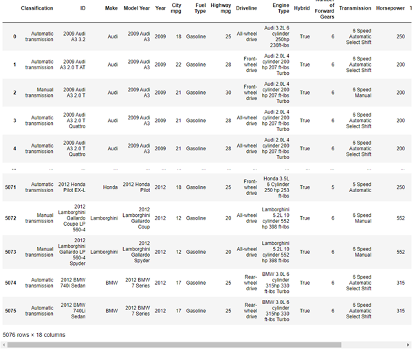
In this case we would like to create a report using some of the data.

The limitation of this is that, whilst they can create very useful displays of data, these graphs still need to be exported and manually organised in presentations or reports. This is where PyBloqs comes in. Using the framework, we can enter a few parameters to instruct the system to automate the exporting process.

First, we will create a plot using this Highcharts AP I :

from pybloqs import Block
from pybloqs.plot import
Chart, Column, Plot, Series, XAxis, YAxis
title_text = "Fuel types as a percentage of available cars by year"
title = Block(title=title_text)
year_fuel_count = df.value_counts(["Fuel Type", "Year"]).unstack(level=-1).fillna(0).astype(int
)
year_fuel_count_plot = Plot(
    year_fuel_count.T, 
    Column(stacking="percent"), 
    Chart(zoom_type="xy"),
    XAxis(title=dict (text="Year")), 
    YAxis(title=dict (text="Percentage")),
    title=title_text,
)
year_fuel_count_plot

The Highcharts API used is a Python wrapper on the official JS Highcharts API, as there is no official Python version. This outputs the following chart:

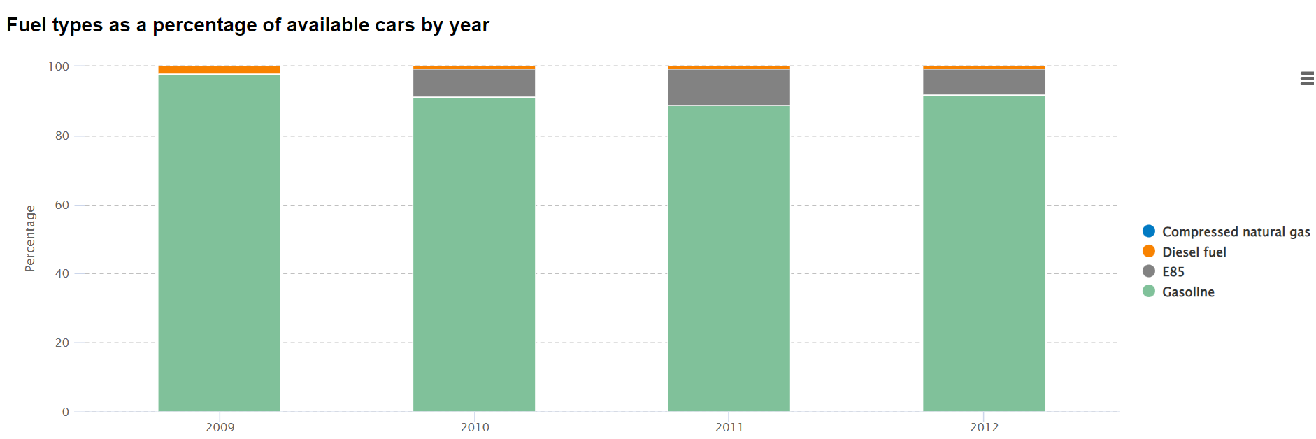
In this example, we have taken the data in the table above, and used PyBloqs to create an interactive bar chart. In this use-case, the information is clearly laid out, and we can hover over the bars or select different categories to drill-down into the information, or tailor it towards different audiences.

As Plotly is a Python library, we just wrap the fig output with a pybloqs.Block

import plotly.express as px

fig = px.scatter(df, x="Horsepower", y="City mpg", title="Horsepower - City mpg")
hp_vs_mpg_plot = Block(fig)

This creates a plot that looks like this:

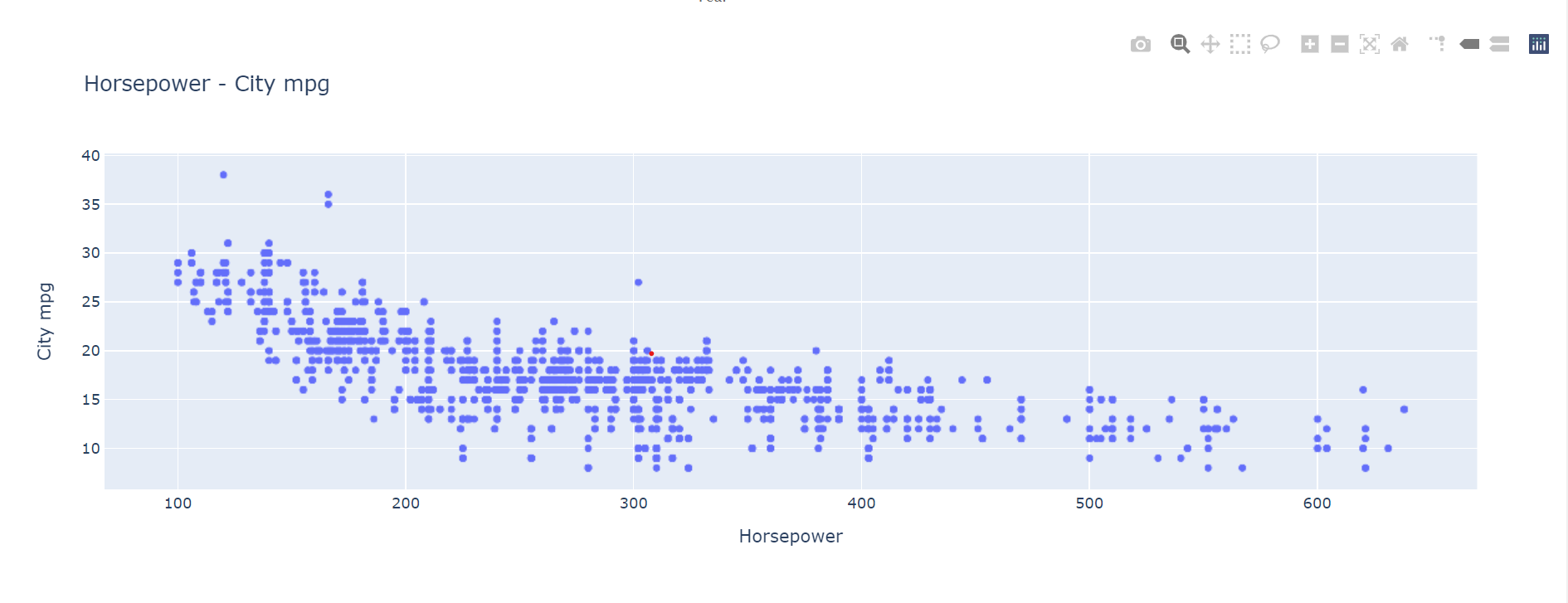
The advantage of an output like this is that it allows the end user to identify specific outliers from complex data at a glance: all that is required is to hover over a specific point. The user can also utilise any of the additional data analysis tools offered by a Plotly output, zooming in, comparing and isolating specific data points.

Whilst this is useful, there is something else to consider. Reports don't just have plots: they also normally contain tabular data. PyBloqs makes it easy to manage the formatting of tabular data that is sourced from a pd.DataFrame. For example, we are easily able to add date, heatmap, and conditional formatters to make our table more visually informative:

import pybloqs.block.colors as colors
from pybloqs import HTMLJinjaTableBlock
pybloqs.block.table_formatter_builder import CommonTableFormatterBuilder

top = df.groupby("Make").head(1)
top = top.loc[top.Make.str.match("Mercedes$|BMW$|Volkswagen$|Mitsubishi$|Toyota$|Honda$|GMC$|Chevorlet|Buick")]
top = top.reset_index().drop(["index", "ID"], axis=1).sort_values(by=["Torque"])
fmt = (
    CommonTableFormatterBuilder(top, table_width=None, font_size=14)
    .date_columns(columns=["Year"])
    .hide_columns(columns=["Make", "Hybrid", "Fuel Type", "Engine Type", "Transmission"])
    .heatmap(columns=["Horsepower"], min_color=colors.GREEN, max_color=colors.HEATMAP_RED)
    .divider_line_vertical(column="Horsepower")
    .threshold(column="Torque", threshold_column="Horsepower")
    .color_background_conditionally_matching(value="All-wheel drive", color=colors.BLUE)
    .color_background_conditionally(condition=Lambdav: v > 5, color=colors.YELLOW, columns=["Number of Forward Gears"])
)
table_block = HTMLJinjaTableBlock(top, formatters=fmt.formatters, use_default_formatters=False, title="Cars with high horsepower")
table_block

This code block outputs the following:

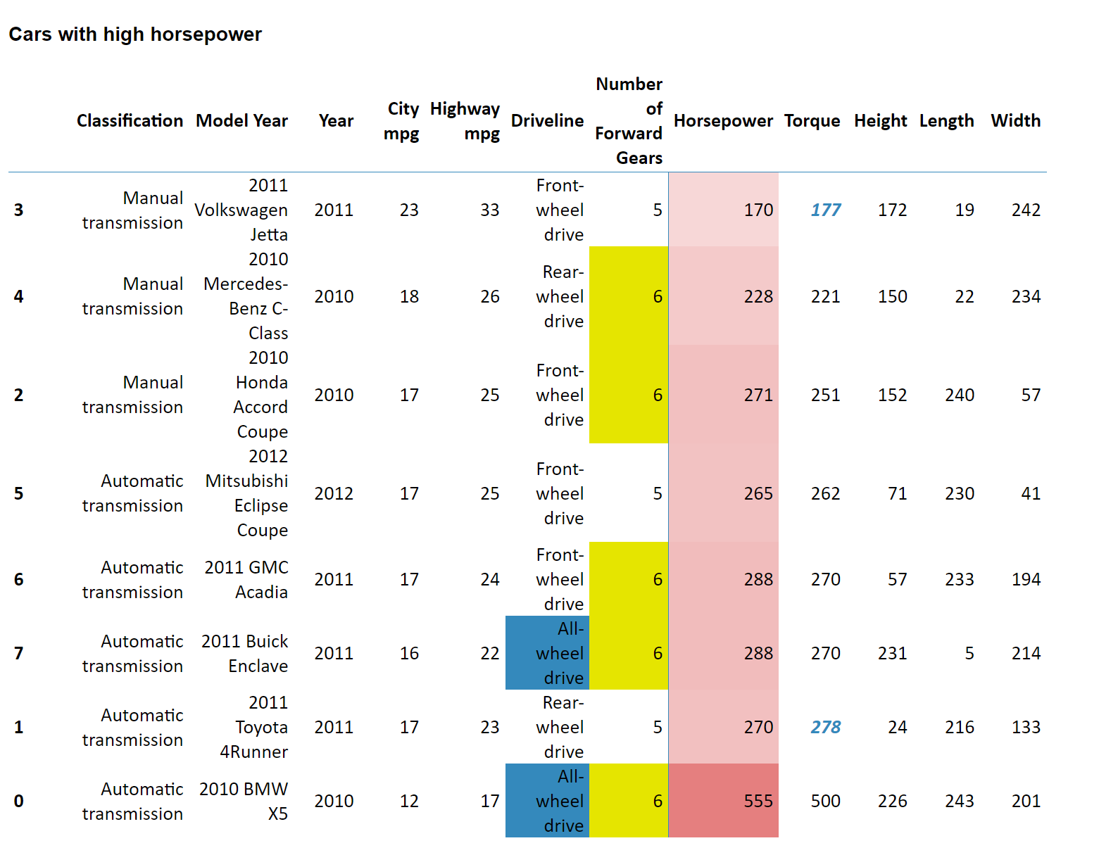
As seen in the code, we can decouple the formatting from the underlying data, such as hiding irrelevant columns. We also apply the builder pattern to streamline the syntax.

However, a few disparate plots and tables do not make a report. To finalise, we can assemble the plots together into a report and render it as an interactive HTML document. PyBloqs also supports rendering to PDF - this outputs the HTML as static images and searchable text within a file.

from pybloqs import Grid

report = Grid([year_fuel_count_plot, hp_vs_mpg_plot, table_block], cols=2)
report.show()
report.save("Car report.html")

And the output can be found here: car report.html

As you can see, this report is pretty simple. The beauty of PyBloqs is in its convenience. Each block of data can be manipulated and output in different ways, depending on what is required. A complex report containing pages of analysis for staff engineers can be created using the same framework as a simple, bare-bones document for presentation to a management committee. Really, the limitation is your own creativity.

We hope that this quick run through has piqued your interest. If you’d like to explore using PyBloqs yourself, please see the documentation here:

https://pybloqs.readthedocs.io/en/latest/

https://github.com/man-group/PyBloqs

If you have any questions, please reach out to us here. https://twitter.com/ManQuantTech