You're Fired! When Do You Sack the Fund Manager?

To read the full academic paper, please visit: https://papers.ssrn.com/sol3/papers.cfm?abstract_id=3583864

Introduction

When evaluating managers or strategies, investors pay close attention to the maximum drawdown, or the largest peak-to-trough return over the life of an investment. For example, for hedge fund investments, money is often pulled out when a threshold for the maximum drawdown is crossed. The maximum drawdown statistic is appealing, as it is unambiguous in its calculation and captures the most unfavourable investment outcome: buying at the peak and selling at the bottom.

The maximum drawdown statistic is different from other metrics such as volatility and downside measures like skewness or semi-variance in that it crucially depends on the order in which the returns occur. In the first part of this paper, we conduct a simulation study to determine the sensitivity of the probability of reaching a given maximum drawdown threshold to key assumptions. We call these the ‘drawdown Greeks’.

Next, we introduce a framework to decide whether to replace a manager (or strategy). This decision will be subject to two types of errors: a Type I error of replacing a good manager and a Type II error of mistakenly not firing a bad manager.¹

We have not tried to identify the impact of drawdown rules on manager behaviour. But we are very aware that the presence of a ‘drawdown rule’ will itself cause managers to act differently – nobody likes getting fired. From this perspective, a drawdown rule might be considered to have some similarities to volatility scaling; managers who show behavioural aversion to being fired will reduce risk near down the drawdown limit. As such, drawdown rules might be considered ‘poor man’s volatility scaling’.

Drawdown Greeks

The key drivers of the maximum drawdown that we identify are: the evaluation horizon (time to dig a hole), Sharpe ratio (ability to climb out of a hole), and the persistence in risk (chance of having a losing streak).

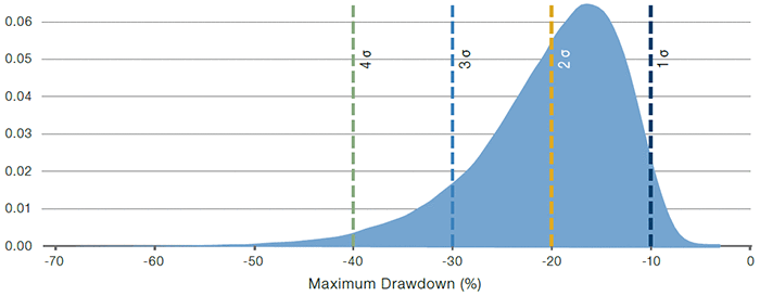
We start with a simple setting of normal, independent and identically distributed (‘IID’) monthly returns.² Figure 1 shows the probability distribution of the maximum drawdown statistic for our baseline case: 10-year time window, 10% annualised volatility, 0.5 annualised Sharpe ratio, where each parameterisation is evaluated with 100,000 simulations of monthly returns for the evaluation window.

We highlight with vertical lines maximum drawdown levels of 1, 2, 3 and 4 annual standard deviation (or sigma) moves, corresponding to -10%, -20%, -30%, and -40% drawdown levels. The associated probability of reaching a maximum drawdown of that level or worse is given by the area under the curve to the left of the associated vertical line. These are 97.1%, 43.0%, 9.9% and 1.5% for 1, 2, 3 and 4 sigma levels, respectively. So in almost half of the cases, one reaches a drawdown of two full annual standard deviations (or -20%) over the 10-year period, even though the annual Sharpe ratio is a respectable 0.5. In 1-in-10 cases, one even reaches a drawdown of three full annual standard deviations (or -30%).

Figure 1. Probability Distribution for the Maximum Drawdown Statistic

Source: Man Group. For illustrative purposes.
The figure shows probability distribution for the maximum drawdown statistic using normal, IID monthly returns over a 10-year window with a 10% annualised volatility and 0.5 annualised Sharpe ratio (the baseline case). The vertical, dashed lines correspond to drawdowns of size 1, 2, 3 and 4 annual standard deviations.

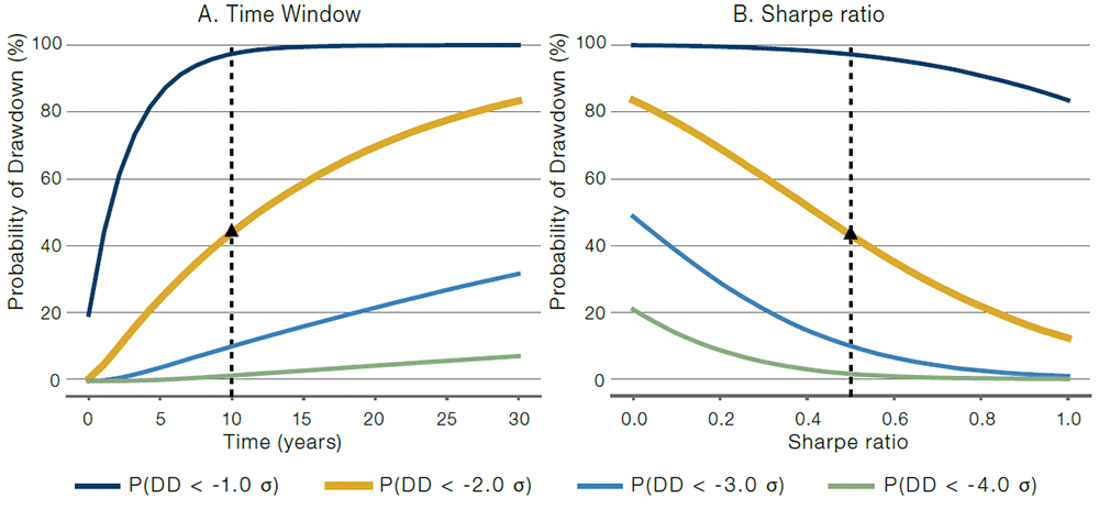
Next, we consider how deviations from the baseline case assumptions impact the probability of hitting a drawdown level. We modify the following assumptions at a time: (A) time window, 10 years baseline and (B) annualised Sharpe ratio, 0.5 baseline. The results are shown in Figure 2.

Figure 2. Sensitivity of the Probability of a Maximum Drawdown to Key Parameters

Source: Man Group.
The figure shows probability of reaching a maximum drawdown of 1, 2, 3 and 4 sigma (annual standard deviations). In all cases returns are normal and identically distributed. In the different panels, we vary the (A) time window and (B) Sharpe ratio. The vertical dashed line corresponds to the baseline case of 10% annualised volatility, 10-year window, 0.5 annualised Sharpe ratio and 0.0 autocorrelation.

The orange line in Figure 2 represents the probability of a maximum drawdown that is -2 sigma (annual return standard deviations), or worse.³ This value is 43% for the baseline case (indicated by the vertical dashed line in Figure 1).

Panel A shows that the probability of hitting a certain drawdown level naturally increases as a return stream is evaluated over a longer window. We use a baseline case of 10 years.

In Panel B, we vary the Sharpe ratio, while holding the constant standard deviation of returns. In the default case, we have an annualised Sharpe ratio of 0.5. The impact of Sharpe ratio on the probability of reaching a certain maximum drawdown level is large, which is intuitive. It is exactly this effect that investors using drawdown rules are hoping to isolate – the low Sharpe ratio managers will be removed by the presence of the rule.

We also find that non-normal, but still time-independent, returns – for example the occasional gap move down – only matter much when they are large compared to what we generally observe for a range of financial markets. The reason is that with independent returns, the central limit theorem kicks in: multi-period returns start to look more normal as one increases the number of periods. As a robustness check, we simulated from historical US equity returns (block bootstrap) rather than from a normal distribution, and we found qualitatively similar results to those shown in Figure 2.

Manager Replacement Rules

So, what performance statistics are the most informative for deciding whether to replace a manager?

To answer that question, we first we assume there are two types of managers:

• Good: producing returns with an (expected) annualised Sharpe ratio of 0.5; and
• Bad: producing returns with an (expected) zero Sharpe ratio.

We also recognise that the decision to replace a manager will be subject to two types of errors:

• Type I error: replacing a Good manager;
• Type II error: not replacing a Bad manager.

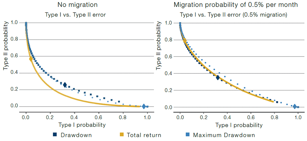
Figure 3 shows the tradeoff between the two error types for three rules applied after a 10-year observation window:

• Total return over the 10 years;
• Drawdown level at the 10-year point;
• Maximum drawdown during the 10-year period.

Each dot in Figure 3 corresponds to a different cutoff value for the respective statistic. A larger diamond highlights the case where we use -10% (-1 annual standard deviation) as the cutoff value for each statistic.

In the left panel of Figure 3, we assume we have a pool consisting of 50% Good (Sharpe ratio 0.5) and 50% Bad (Sharpe ratio 0.0) managers with returns that are normal, IID and with an annualised standard deviation of 10%. Crucially, we assume managers are of constant type. Here, it is clear that classification based on the total return leads to a better Type I/Type II tradeoff than using a drawdown-based rule, as the curve is closer to the origin (low Type I and Type II errors).

In the right panel of Figure 3, we assume all managers start off as Good, but that they migrate to Bad at a constant monthly rate over time. The assumed monthly migration rate is 0.5%, which means that after 10 years, around 45% of managers have migrated from Good to Bad. These assumptions are motivated by the fact that in practice, managers or strategies can migrate from Good to Bad because of structural market changes, increased competition for the strategy style employed, staff turnover or a fund accumulating too many assets. Now, the drawdown- and total return-based rules are similarly effective. This is a big change from the case of constant manager types (left panel), where the total return-based rule was superior. The pick-up in the appeal of drawdown-based rules here is intuitive, as they put more emphasis on recent history, and so are more tailored to the possibility of a migration from Good to Bad.

Figure 3. Efficacy Classification Rules With a 10-Year Horizon

Source: Man Group.
We show the Type I error (mistakenly replacing a Good manager) and Type II error (mistakenly keeping a Bad manager) for three replacement rules. Evaluation takes place after observing 10 years of monthly data. In the left panel, the pool of managers consists of 50% Good and 50% Bad managers. In the right panel, all managers start off as Good, but each month there is a 0.5% chance of migrating to a Bad manager type. Good and Bad managers have a Sharpe ratio of 0.5 and 0.0 respectively. Returns are normal, IID, with 10% annualised volatility for both manager types. Different observations correspond to different cutoff values for the replacement rule, with a diamond corresponding to a -1 sigma cutoff.

As can be seen in the figure, a -10% cutoff value (represented by the big diamonds in the plot) leads to very different Type I error values. It is, for example, much more common for the drawdown level to hit -10% than it is for the total return to reach -10%. In fact, every time the total return hits -10%, the drawdown must also be at least as bad as -10%. The reverse does not hold.

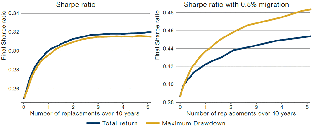
In reality, the decision to replace a manager is not done once, at the end of a long observation window, but intermittently. For example, some multi-manager hedge funds state very clearly upfront at what drawdown level a portfolio manager is fired. Interestingly, typically a constant cutoff value is used, rather than allowing for larger drawdowns when a manager has been running for a longer time. The reasons for this may be behavioural – in other words, the rule is intended to alter manager behaviour whether the manager has long tenure or not. Figure 4 compares the efficacy of a total return and maximum drawdown rule to replace managers, where we make the same assumptions on manager types as before in Figure 3, but where an investor evaluates managers monthly for a 10-year period.

Of course, simply comparing Type I and II error rates is not sufficient in the case of monthly evaluation, because it also matters how fast a bad manager is replaced. Instead, Figure 4 shows the Sharpe ratio over a 10-year window, with managers being replaced when they hit the threshold value.

Additionally, replacing a manager can be costly because it requires due diligence into new managers, involves legal costs, and resets the high water mark in case of performance-fee charging hedge funds. For this reason, in Figure 4, we plot the resulting Sharpe ratio when using the two replacement rules as a function of the average number of replacements during the 10-year window. To this end, we vary the cutoff value, and, for each value, plot the average Sharpe ratio as a function of the total number of replacements over the 10-year period.

In the left panel of Figure 4, we see that in case of constant manager types, the total return is better than the drawdown-based rule. This is consistent with the left panel of Figure 3. Again, the intuition is that the total return is an efficient statistic for estimating a manager’s average return, while the drawdown statistic is path-dependent and so more wasteful in its use of historical return observations.

In the right panel of Figure 4, we see that in case of a manager migrating from Good to Bad, a drawdown-based replacement rule is more effective in that it results in a higher Sharpe ratio for a given number of replacements over 10 years. The superior performance of the drawdown-based rule is intuitive, as it more naturally picks up on recent, sudden drop-offs in performance.

Figure 4. Efficacy of Replacement Rules With Monthly Evaluation

Source: Man Group.
We show the average Sharpe ratio over a 10-year window, with a monthly decision to replace managers based on either a total return-or drawdown-based rule. In the left panel, the pool of managers consists of 50% Good and 50% Bad managers. In the right panel, all managers start off as Good, but each month there is a 0.5% chance of migrating to a Bad manager type. Good and Bad managers have a Sharpe ratio of 0.5 and 0.0 respectively. Monthly returns are normal, IID, with 10% annualised volatility for both manager types. We vary the cutoff value used in the replacement rule and plot the average Sharpe ratio against the average number of replacements.

Conclusion

So, what type and size of drawdown should cause you to change investment manager? We draw five main conclusions.

First, know your stats. Drawdowns are easy to compute. However, it is challenging to estimate the probability of hitting a certain drawdown level.

Second, a pre-set drawdown rule may prevent peak risk taking. Taking risk in bursts will increase the probability of hitting a certain drawdown level, relative to more constant risk taking. Hence, clearly communicated drawdown limits can motivate a manager to take more even risk over time.

Third, think in terms of the relative cost of Type I and Type II errors. If hiring a manager is a costly endeavor, Type I errors (booting good managers) are costly. If a bad manager just adds noise (has a Sharpe ratio of zero) in an otherwise diversified portfolio, and if ample cash is available, some Type II errors (keeping a bad manager) may not be that bad. However, if bad managers have a substantially negative Sharpe ratio (e.g., because of transaction costs or because they unwittingly take the other side of the trade of some shrewd investors), Type II errors become much more of a concern.

Fourth, look at both total return and drawdown statistics. Total-return (or Sharpe-ratio) rules are best at measuring the constant ability of a manager to create positive returns. Drawdown-based rules, on the other hand, are better suited to deal with a situation where a manager abruptly loses their skill. In reality, the two are complementary.

Fifth, consider a time-varying drawdown rule. The probability of hitting a certain drawdown level naturally increases over time, even if a manager continues to be of the same type, generating returns from a constant distribution.

Harvey is at Duke University, the National Bureau of Economic Research and is an adviser to Man Group plc. The other authors were at Man Group plc during this research. The authors would like to thank Nick Barberis, Anthony Ledford, Matthew Sargaison, and Rikiya Takahashi for valuable comments. Please direct correspondence to: Otto.VanHemert@man.com.
1. See also Harvey and Liu (2020) for a discussion of the tradeoff between Type I and Type II errors, as well as their differential costs.
2. Our analysis is based on monthly, rather than daily, return data for two reasons. First, we think investment and allocation decisions by large institutions are more likely to take place at a monthly frequency. Second, returns at the daily frequency are harder to model as they are influenced by a pronounced intra-month variation in the news flow; e.g., bigger moves on the day major economic news is released. Monthly returns are somewhat better behaved, as they reflect the combination of both high- and low-news days. The more complicated case of daily drawdown evaluation and replacement decisions is left for future research.
3. Both the variable we vary on the horizontal axis and the -2 sigma cutoff are based on the (ex-ante) standard deviation for the return process. Probabilities (vertical axis) are based on average realised values.