Questioning Quality

Introduction

The Growth versus Value paradigm has been discussed extensively over the course of 2020. This year is just a microcosm of the past decade as far as the relationship between the two factors goes, with every analyst and fund manager (including ourselves) opining on the market’s seemingly insatiable appetite for growth at any price to the detriment of value.

There’s another pillar of factor investing, though, whose travails have been underreported, but where we perceive similar evidence of ‘alpha decay’: Quality. Though the definition of Quality varies by investor, some of its most visible measures have seen their excess returns eroded in the years following the Global Financial Crisis (‘GFC’), especially within US stocks. Here, we look at the reasons behind this underperformance, attempting to differentiate between the general market environment and performance lost due to the potentially self-inflicted wounds of model overfitting and quant crowding.

While there are a wide range of metrics that could form part of a well-rounded assessment of a company’s quality, we focus here on connecting the designation of quality to the concept of ‘bad’ and ‘good’ growth. What we call bad growth is driven by balance sheet expansion. Good growth comes from enhanced profitability rooted in competitive advantage. It is, we believe, crucial to understand the interplay of these different types of growth and their impact on valuations in order to achieve a more nuanced assessment of the performance of the quality factor in the decade since the GFC.

While expansionary periods tend to lessen the penalties for bad growth and the rewards for good growth, we cannot blame Quality’s decay in the US solely on the unprecedented duration of the post-GFC expansionary regime. It’s striking that US companies with high levels of asset growth have been able to preserve their relative valuations more effectively in the post-GFC market environment than in prior periods, creating an alpha headwind of 3-5% annually to the performance of factors targeting the bad growth anomaly. In this article, we will attempt to understand the drivers of this valuation effect by examining crowding, the lack of mean reversion in profitability and the payoff link between anti-asset Growth factors and Value.

We note that it appears that network effect-driven competitive advantage¹ may be the straw that broke the back of the bad growth thesis in the post-GFC period. FAANGM² stocks, in particular, have succeeded in maintaining strong levels of asset growth while also achieving impressive profitability. Apparently, network-based advantages are difficult to dislodge.

Profitability-driven good growth has been one of the better-performing factors globally over the last decade, in part due to investors’ preferences for growth and safety in the post-GFC era and the manner in which highly profitable companies have been able to maintain their competitive advantage. However, in the US at least, companies with superior returns on equity haven’t delivered as much fundamental growth compared to their less profitable peers over this past decade as in prior periods, creating a drag on the factor’s performance of 2-4% annually. Somewhat surprisingly, profitability-driven factors may be the most sensitive to crowding, at least according to our statistical measurement.

Factor Performance: E&I Quality in Sharper Decline Than Profitability

Let’s begin with some basic performance observations. Within the Quality factor, models targeting earnings and investment (‘E&I’) quality have exhibited a sharper decline globally than those based on profitability, which have experienced a recent performance revival. E&I models seek out companies with shrinking balance sheets based on the observation that investors tend to overpay (at least historically) for investment-driven growth (i.e., bad growth). A growing balance sheet may be symptomatic of rising accounting accruals as well, which can drive less persistent and more manipulable future earnings that investors may not properly discount in valuation.

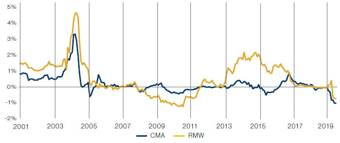
Figure 1 plots the trailing 10-year Sharpe ratio of the Fama-French CMA (‘Conservative Minus Aggressive’) asset growth factor, highlighting the decline in the factor’s performance by region following the aftermath of the GFC.³ We can think of asset growth as a ‘kitchen-sink’ E&I factor since it captures changes on both the left- and right-hand sides of the balance sheet (assets = liabilities + book value, after all), including growth in line items such as: accounts receivable; property, plant and equipment; net debt; retained earnings; and net dollars of share issuance.^4,5

Figure 1. Trailing 10-Year Sharpe Ratio of CMA

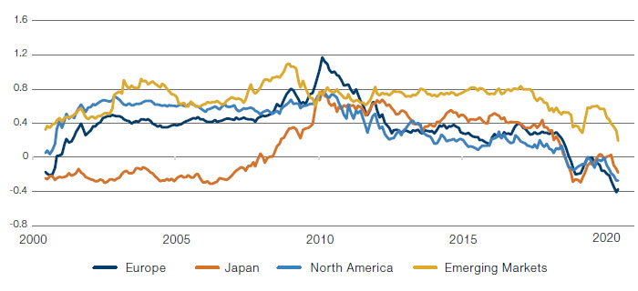
Source: Tuck at Dartmouth Kenneth French Data Library; as of 30 June 2020.
CMA is a proxy for E&I Quality.

On the other hand, Profitability (a driver of good growth) has been one of the better-performing factors globally over the last decade. In the post-GFC market environment, investors have targeted Growth and Safety factors like Low Volatility and Profitability. Figure 2 plots the trailing 10-year Sharpe ratio of the Fama French RMW (‘Robust Minus Weak’) Operating Profitability factor. North America stands out as a modest exception, where the Sharpe ratio has been flat to down during the last decade.

Figure 2. Trailing 10-Year Sharpe Ratio of RMW

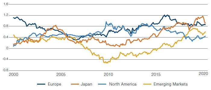
Source: Tuck at Dartmouth Kenneth French Data Library; as of 30 June 2020.
RMW is a a proxy for profitability.

Two Facets of the Quality Thesis: Good and Bad Growth

The Quality story is very much tied to Growth, and so far we have made assertions about good versus bad growth without much theoretical justification. Foundations are important if we hope to understand recent performance drivers and make some educated guesses about the future. Much like a money manager facing the tension between alpha and capacity, the CEO of a corporation must optimise the trade-off between profitability and growth. Retaining more earnings/cashflows or adding equity capital today necessarily places pressure on tomorrow’s profitability. Debt enhances equity returns but increases the chance of bankruptcy and makes the same demand on a firm’s ‘competitive capacity’ as equity.

We can trace the mechanics of growth through the evolution of a firm’s net operating assets and book value.⁶ Net operating assets grow through higher returns on assets in place (e.g., RNOA/ROIC) or increased retention of operating profits that are directed to future capital investments (or retirement of operating liabilities) rather than distributed as free cash flows to asset holders. In related fashion, the firm may grow book equity per share by increasing its profitability per unit of capital (e.g., ROE), retaining more of its earnings for future investments rather than pay dividends to shareholders, or issuing/buying back shares depending on the market’s pricing of its stock.

The thesis behind the quality alpha generating process is that investors overpay for growth driven by balance sheet expansion and underpay for the ‘alpha’ of per-unit profitability. A firm with a growing balance sheet overinvests and eventually loses some portion of its competitive advantage, either through direct competition or overgrowing its optimal size.⁷ This loss is eventually manifested in a drop in multiple. In the end, what was gained in growth was subsequently more than lost in multiple contraction. And, for their trouble, equity and asset holders have sacrificed near-term dividends and cash flows. In contrast, increasing or at least maintaining core profitability relative to one’s competitors is a seemingly productive proposition rooted in improving operational efficiency and sustainable competitive advantage and (holding all else constant) yields higher returns for share or asset holders.

If we look back before the 2010s, this thesis held in practice across large- and smallcap stocks, irrespective of the specific measure used for growth (e.g., growth in assets, operating assets, non-current operating assets, book value) or profitability (e.g., ROE, ROA, RNOA, Gross Profits of Assets). So, what’s happened in the last 10 years to challenge the thesis for bad growth and weaken the returns to good growth in the US?

Economic and Market Backdrop Cannot Completely Explain Alpha Decay of Quality

The macro- and micro-economic landscape of the last decade has differed meaningfully from the historical periods that academics and practitioners used when developing their initial Quality models in the mid-1990s and early 2000s. One obvious difference is the unprecedented duration of the post-GFC economic expansion in the US, which lasted 128 months, beginning in July 2009 and ending abruptly in March 2020 due to the Covid-19 pandemic. Historically, E&I Quality and Profitability factors have been more productive in periods of economic contraction.

We explore this in Figure 3 by delving deeper into history while limiting ourselves to US stocks and splitting the performance of each FF factor between recessions and expansions that occurred prior to July 2009.⁸ Of the factors, RMW (a proxy for Profitability) and CMA (a proxy for E&I Quality) exhibit the strongest risk-adjusted performance of all factors in recessions, while still posting competitive numbers in expansions. We need to be careful about over-extrapolating these findings. Much of CMA’s countercyclical benefit came in the recessions of the 1970s and 1980s, while RMW was relatively strong during the collapse of the TMT bubble and GFC. Our broader point, however, is that for all non-market related factors, the realised Sharpe ratios and returns of the last decade’s expansion fall well below previous expansionary periods, indicating that alpha decay for Quality (and Size and Value) cannot be explained entirely by the post-GFC economic regime.

Figure 3. US Fama-French Factor Performance

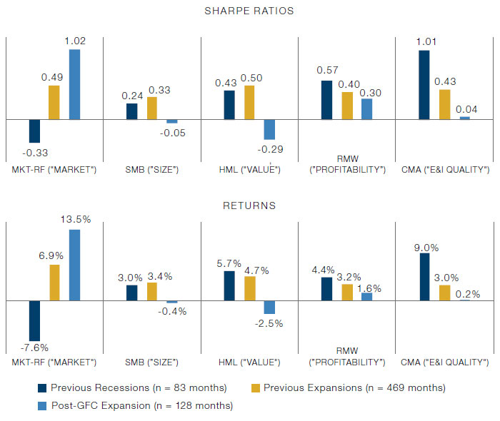
Source: Tuck at Dartmouth Kenneth French Data Library; between July 1963 and February 2020.

While the post-GFC expansion was the longest in the history of the US, the levels of GDP and employment growth ran at one-third to half those of previous expansions, keeping interest rates low for the entire period. Low rates, coupled with psychological scarring from the GFC, drove investor demand for two factors: growth and safety. The former provides a natural headwind to anti-asset growth factors like E&I Quality (e.g., CMA), while both should benefit profitability-based Quality signals (e.g., RMW, ROE). Based on recent Federal Reserve signaling, we don’t expect the interest rate environment to change any time soon, and the Covid-19 crises is clearly not a salve for investor risk aversion. Notwithstanding headwinds and tailwinds from investor demand, we will show later that a significant portion of alpha decay can be explained by a deterioration in the delivery of fundamental growth relative to prior periods in the case of profitability and a lack of multiple expansion when it comes to E&I quality.

It is worth discussing other differences in the recent environment relative to the deeper history used in academic and practitioner back-tests. General improvement in corporate governance and accounting oversight (including the Sarbanes-Oxley legislation) may have weakened the hypothesis driving the accrual components of earnings quality. Generally accepted accounting rules may not fully value investments in intangible assets such as R&D, brand and organisational talent development, which have become increasingly important. In addition, the business environment may favour higher persistence in relative profitability with the rise of a network effect-driven competitive advantage and with enforcements down significantly from the 1940s-1970s ‘Golden Era’ of antitrust.⁹ There is quite a bit to unpack here, and we may not cover each of these dimensions adequately. We will focus on a few things we can measure directly, namely signal stretch, industry effects and persistence in relative profitability.

Signal Stretch Did Not Meaningfully Narrow

A basic diagnostic for forecasting model efficacy is signal ‘stretch’ – the raw distance between high- and low-ranked stocks. We often apply the stretch concept in our evaluation of the opportunity for value investing, but it is a concept that is applicable more broadly. The premise of the stretch is simple: the wider the distance, the more actual dispersion there is in the metric and therefore the easier it is for the model to discriminate between stocks. For asset growth and profitability models, the distance is purely fundamental; there are no market prices in their construction. It could be that the environment of the last decade has driven firms to coalesce around roughly the same levels of asset growth and/or competitive pressures have narrowed the relative differences in ROE. With closer reflection, though, this does not seem to be the case.

Figure 4 plots the various percentile breakpoints for both models by month for the top 1,500 companies in the US by market cap from 1995 to 2019. There does not appear to be an unusually narrow or wide stretch in either asset growth or ROE in the last decade of the data. For asset growth, the distance between the 75th and 25th percentiles drops from 20% in mid-2008 to 16% at the end of 2019. The stretch over the last 20 years is well below the 35% level seen in 2000, when the anti-asset growth factor performed quite well, posting a 35% alpha (coincidentally the same number) for the year. Median return on equity has been steady at 12-13% post GFC with a stretch of about 15%.¹⁰ We’ve added a 90th percentile breakpoint for ROE to highlight that the stretch between the average and the most profitable companies has widened. We will touch briefly on this effect when we discuss industry dynamics and profit persistence.

Figure 4. US Top 1,500 Signal Breakpoints by Month

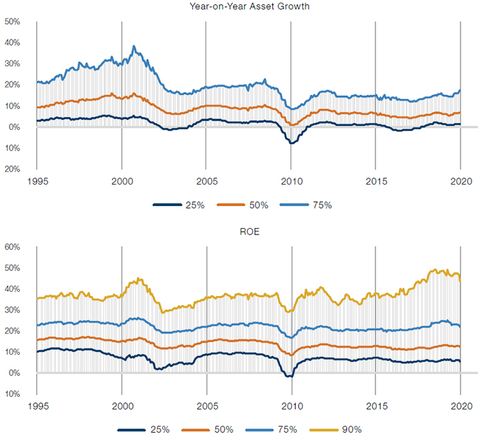
Simulated past performance is not indicative of future results. Returns may increase or decrease as a result of currency fluctuations.

Source: S&P Global and Man Numeric; between 1995 and 2019.
Simulated performance data and hypothetical results are shown for illustrative purposes only, do not reflect actual trading results, have inherent limitations and should not be relied upon. Please see the end of this paper for additional important information on simulated results.

Figure 4 also reveals that median corporate balance sheet growth is down (despite low interest rates) from 9% per year in the 2000s to 6% in the 2010s, indicating that aggregate E&I Quality as measured by asset growth has improved. There are several potential drivers of depressed asset growth including better investment discipline in the post-GFC environment, improved accounting oversight, and the shift of corporate investment from tangible to intangible assets.

This last point is interesting since it is linked to Value’s struggles as well. Accounting rules require intangible investments to be expensed rather than capitalised in the period incurred, biasing measurements of assets or book value downward from a firm’s true value as well as undercounting current profits. This has been one of the arguments put forward for the recent poor performance of deep value metrics like book-to-price and for the potential benefits of income statement items such as gross profits that do =not penalise corporations for R&D and SG&A spending.^11,12 These lines of argument assume, of course, that such investment in intangibles ultimately bear fruit for the firm.

Industry Effects Matter and Are Important to Control For

It might be thought that these accounting rules favour knowledge economy stocks over more traditional businesses in the measurement of asset growth. This effect is counteracted, though, by fundamental changes that have taken place in the post-GFC landscape, most notably the significant (relative) shrinking of assets in the energy and diversified financial industry groups. Whatever impact intangible accounting biases may have, the two industry groups with the largest asset growth rates in the 2010s have been knowledge economy industries: software and pharma/biotech.

Figure 5 plots the median trailing 12-month ROE (y-axis) versus the median annual asset growth rate (x-axis) by industry group averaged from 2010-2019.

Figure 5. Median Trailing 12-Months ROE Versus Asset Growth by Industry Group

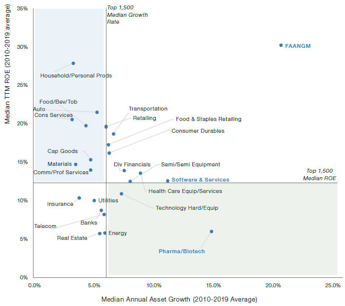
Source: S&P Global and Man Numeric; between 2010 and 2019.

Industry groups in the top left quadrant of the graph are considered higher quality in both E&I Quality (below median asset growth) and profitability (above median ROE).¹³ Groups in the bottom right would be in the opposite camp. A CEO would like their company to be in the top right quadrant, the best of all positions, where it would be classified as a highly profitable growth company – precisely the location of the FAANGM¹⁴ juggernaut. We’ve combined the balance sheets and income statements of the FAANGM firms to form a single company, which posted an astonishing 30% average ROE and 20% average annual growth in assets over the last 10 years. These stocks are strong counterfactual examples of the bad growth thesis and a driving force behind the decay of E&I Quality.

Persistence of Relative Profitability Has Increased

In addition to investor preference for Growth and Safety factors in the last decade, another element that has provided a tailwind to Profitability (and headwind to Value) has been the competitive environment, where, by our estimates, the rate of mean reversion in company profitability is slowing. Companies with above-average profitability appear to have become more likely to maintain that position year-over-year. Likewise, companies with below-average profitability may find it difficult to dig themselves out of their relative holes. To measure profit persistence, we fit the following first-order auto-regressive (i.e., AR(1)) model cross-sectionally each month from January 1995 to June 2019 (using data through June 2020) for stocks in the top 1,500 by market cap in the US:

rank(ROE_t+12)= a₀ + a₁rank(ROE_t)+ϵ_t+12

One-year ahead profitability is a function of current profitability. The coefficient, a₁, measures the impact of ongoing competitive pressure on profitability (i.e., a ‘fade factor’ expected to be between 0 and 1). It may be interpreted as a measure of persistence – a larger value implies less mean reversion across stocks next year. To mitigate outlier effects and control for macro cycles, we standardise ROE crosssectionally each month (leading to an intercept a₀ = 0 by construction). We fit another version where we control for industry group effects, which models the average rate of reversion of each stock to its industry group average ROE.

In Figure 6, persistence in relative profitability is trending upward over the period, whether to market-wide or industry group averages. Some of these effects may be driven by the absence of a recession in the post-GFC period until recently, and we will need to see the ultimate impact from the Covid-19 crisis as new profit data becomes available. Nevertheless, competitive advantage, it seems, has been easier to maintain today. Indeed, a recent study has shown that over 75% of US industries have experienced an increase in concentration levels since the late 1990s and that firms in industries with the largest increases in product market concentration (proxied by sales concentration and the number of publicly traded firms within an industry) have shown higher profit margins and executed more profitable mergers and acquisitions deals.¹⁵

Over the whole sample, our regression coefficients imply that the competitive half-life (i.e., the number of years it takes for a company to revert half-way back to average profitability) has lengthened from 1.5 years (1995-2009) to just over two years (2010-2019).¹⁶ A small shift, yes, but in a direction that implies forecasting relative profitability has become easier not harder. Persistence in relative profitability, which supports premium valuations, may be one of the drivers behind the outperformance of Growth stocks (and struggles of Value stocks) in the last decade.

Figure 6. US Largest 1,500 AR(1) Coefficients

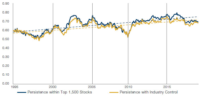
Source: S&P Global and Man Numeric; between January 1995 to June 2020.

Attributing the Returns to Quality

So far, we have made several observations regarding the post-GFC environment. Here, we will link the findings above directly to the returns of E&I quality and profitability. The connection is made through a decomposition of portfolio return across the four drivers displayed in Figure 7: growth in fundamentals, multiple expansion, debt repayment and dividend income.¹⁷

The choice of fundamentals used to measure growth is flexible but does require some sensible link to valuation. The other consideration is around sensitivity to macro cycles, whether recessions or expansions. Items higher in the income statement are more stable year-over-year, while those further down are more representative of short-term earnings power but harder to value around inflections. We’ve selected three proxies for growth in cash flows to asset holders: year-over-year change per share in sales, gross profits, and EBITDA.¹⁸ Finally, given the increasing importance of share buybacks, we report net buyback yield (‘NBY’) in addition to dividend yield.¹⁹ While their impact on share price is hard to attribute, net buybacks may be useful as a forecasting tool in the spirit of dividend discount modelling.²⁰ The effective ‘yield’ of these portfolios is the sum of dividend and net buyback yield.

Figure 7. Total Return Decomposition Framework

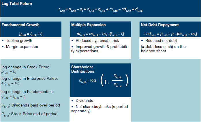
Source: S&P Global, the Center for Research in Security Prices and Man Numeric; as of 9 September 2020.

For our Quality factor tests, we examine year-over-year asset growth (similar to FF’s CMA factor) and trailing 12-month ROE (similar to FF’s RMW factor), for the top 1,500 stocks in the US by market cap from 1995 to 2019. We also look at a Value composite factor to provide an additional comparison.²¹ We remove financials and REITs from the sample, leaving us with 1,150 to 1,250 stocks to choose from each month. Stocks are ranked for each of the three signals after subtracting their respective industry group average score to control for persistent industry differences and macro risks. We form cap-weighted, vintage portfolios each month and study their evolution over the following 12 months. For example, the January 2019 vintage, constructed using data from the end of December 2018, incorporates returns and fundamental changes from January through December 2019. The inputs to the attribution equations above are calculated at the portfolio level. With sector and market cap restrictions, vintage construction versus monthly rebalancing, and industry group adjustments, we expect to see differences in returns compared to FF but with qualitatively similar outcomes.

To orient ourselves, we first apply the attribution to the broader universe of stocks in our study, split between pre- and post-GFC periods. Figure 8 shows that returns are driven predominantly by underlying growth in fundamentals during both periods, while the market of the last decade has enjoyed the benefits of multiple expansion and the lack of a recession until Covid-19. Our last vintage covers returns through December 2019.

Figure 8. US Broader Market (Largest 1,500 ex-Financials/REITs)

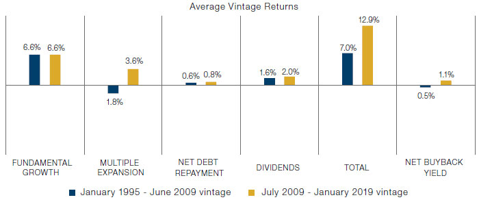
Simulated past performance is not indicative of future results. Returns may increase or decrease as a result of currency fluctuations.

Source: S&P Global, the Centre for Research in Security Prices and Man Numeric; January 1995 to January 2019 Vintages.
Simulated performance data and hypothetical results are shown for illustrative purposes only, do not reflect actual trading results, have inherent limitations and should not be relied upon. Please see the end of this paper for additional important information on simulated results.

For our factor study, we formed three long-short ‘30/30’ portfolios derived from six underlying stock groupings:

• E&I Quality: Short ‘Bad’ Growth = (-) Asset Growth: Long the bottom 30% and Short the top 30% of stocks based on year-over-year growth in total assets;
• Profitability: Long ‘Good’ Growth = (+) ROE: Long the top 30% and Short the bottom 30% of stocks based on return on equity;
• Long ‘Value’ = (+) Value: Long the top 30% and Short the bottom 30% of stocks based on a composite value blend.

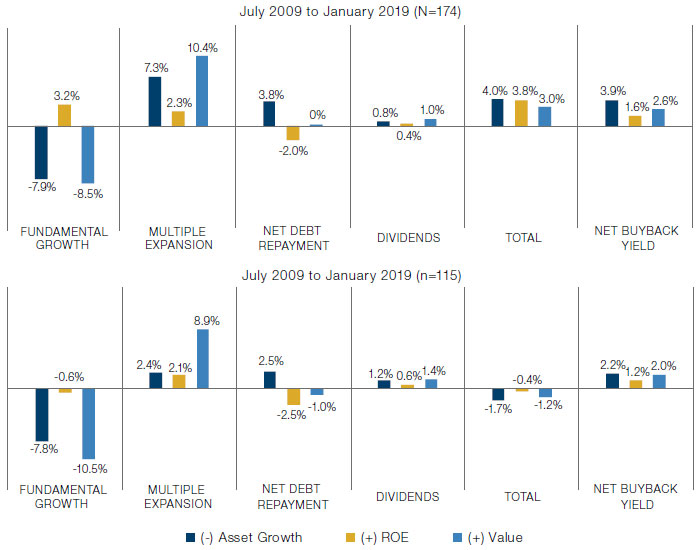
The first panel in Figure 9, covering vintages from 1995 to June 2009, confirms the good versus bad growth thesis. Both Quality strategies generated alpha of ~4% annually but in different ways. The (-) asset growth portfolio exhibited poorer fundamental growth (-7.9% per year) but gained through multiple expansion (+7.3%), debt repayment (+3.8%), and enhanced dividend yield (+0.8%). This portfolio had a 3.9% NBY yield over the period. The (+) ROE portfolio exhibited fundamental growth (3.2%) and multiple expansion (2.3%) that compensated for the additional debt added to support growth. This portfolio, which exhibited above average growth by design, generated less, but still positive, yield in dividends and buybacks totaling about 2%.

Of the two quality factors examined here, the payoff of (-) asset growth is like (+) value’s – driven by poor fundamental growth offset by multiple expansion. The realised returns of the two strategies are correlated. The HML and CMA FF factor returns, for example, have a 68% correlation from July 1963 to through June 2020, the highest pairwise correlation among the five FF factors. Interestingly, Hou, Xue, Zhang (HXZ) argue that investment quality factors like CMA largely subsume value in explaining the cross-section of average stock returns and so do not include value as part of their four model ‘q-factor’ suite of market factor, (-) size, (+) ROE, and (-) asset growth.²²

Figure 9. Average Vintage Returns by Period

Simulated past performance is not indicative of future results. Returns may increase or decrease as a result of currency fluctuations.

Source: S&P Global, the Centre for Research in Security Prices and Man Numeric; as of 9 September 2020.
Simulated performance data and hypothetical results are shown for illustrative purposes only, do not reflect actual trading results, have inherent limitations and should not be relied upon. Please see the end of this paper for additional important information on simulated results.

The second panel summarises the vintages from July 2009 to January 2019 (with returns through December 2019).²³ Here we see a different story. The (-) asset growth portfolio incurred less multiple expansion than in the prior period, creating a headwind of 4.9% per year and negative total returns.

The (+) ROE portfolio was down modestly over the period, driven primarily by lower fundamental growth (3.9% headwind).²⁴ Note the period-over-period differences for the respective standalone FF factor performances for CMA and RMW (not shown) were broadly in line with our quality factors, though the return levels for both FF factors were higher than ours by about 2% annually. This is likely due to the previously mentioned differences in model construction and investable universe.

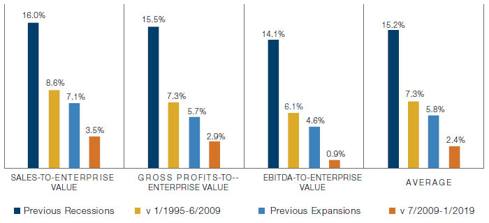
For (-) asset growth, reduced multiple expansion in both the later sample and versus prior expansionary periods holds across each value metric used in the analysis (see Figure 10). So, based on aggregate and specific valuation metrics, it appears that high asset growers (such as FAANGM) have been more effective in maintaining premium valuations in the post-GFC era. The hard part is to understand why. Theories we will explore include the impact of crowding, valuations being justified by profitability, and the outsized impact of a narrow subset of stocks with successful business models that have been rewarded handsomely.

Crowding, the effect of which would be seen mainly through multiple expansion/contraction – as active investors move relative prices higher at purchase and downwards at sale – is one potential driver of premium valuations for high asset growers. The 4.9% alpha headwind from reduced multiple expansion can be attributed as 2.7% due to paying more to put the trade on and 2.2% due to receiving less when taking the trade off in terms of valuation multiples at entry and exit.²⁵

Figure 10. (-) Asset Growth Multiple Expansion Detail

Simulated past performance is not indicative of future results. Returns may increase or decrease as a result of currency fluctuations.

Source: S&P Global, the Centre for Research in Security Prices and Man Numeric; January 1995 to January 2019 vintages.
Simulated performance data and hypothetical results are shown for illustrative purposes only, do not reflect actual trading results, have inherent limitations and should not be relied upon. Please see the end of this paper for additional important information on simulated results.

There is some evidence that these premium valuations are supported by superior profitability in the recent period. The (-) asset growth portfolio benefits from mean reversion in profitability – stocks purchased at the beginning of the vintage improve by about 0.2 to 0.3 standard deviations in relative profitability over the course of the next year (data not shown). This is a key driver of the bad growth thesis. Low asset growers improve fundamentally relative to high asset growers over time. In the post-GFC period, the rate of mean reversion is 70% of prior expansionary periods.

Another (and maybe the easiest) answer to our question about multiples is to attribute the difficulties to the handful of stocks that have had extremely successful business models. Despite the industry adjustments made in our model, the portfolio held 15-20% of its capital short in technology. Removing FAANGM alone would boost vintage returns from -1.7% to +1.1%, a large move for just a few names. To end on a positive note for E&I Quality, investor demand for any type of growth is at potentially all-time highs, motivated by the low interest-rate environment, and one would expect some reversion going forward.

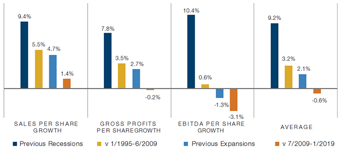
The causes of the decay of the (+) ROE portfolio are a little easier to identify. The lack of relative growth appears central. The alpha headwind from lackluster growth ranges from 2% to 4% if we examine each of our growth metrics independently or compare to prior expansionary regimes only (Figure 11). As an aside, it is interesting that high ROE names provide more relative growth in recessions. We need to be somewhat careful given that only about 10% of the vintage-months were in recession during the prior period, but it’s intuitive that high-quality Growth companies should hold up best fundamentally in adverse economic climates.

Figure 11. (+) ROE Fundamental Growth Detail

Simulated past performance is not indicative of future results. Returns may increase or decrease as a result of currency fluctuations.

Source: S&P Global, the Centre for Research in Security Prices and Man Numeric; January 1995 to January 2019 vintages.
Simulated performance data and hypothetical results are shown for illustrative purposes only, do not reflect actual trading results, have inherent limitations and should not be relied upon. Please see the end of this paper for additional important information on simulated results.

Self-Inflicted Wounds

Confounding our fundamental analysis so far are the actions of systematic equity players, including ourselves. We need to accept that some portion of model decay may be entirely self-inflicted. Two pessimistic scenarios are at play here. First, it is possible that the Quality anomaly never existed in any fundamental sense and was just the outcome of a broad ‘in sample’ fitting exercise with hundreds of academics and practitioners functioning unknowingly as a gigantic, organic machine learning engine. In that scenario, we are now experiencing the true, ‘out-of-sample’ performance of Quality. The second scenario involves crowding, whereby the Quality anomalies are fundamental (or behavioral, take your pick), but their broad adoption by the systematic equity community has arbitraged them away.

Overfitting

The timing around the development of models targeting the Quality anomaly is somewhat damning, with accrual research in the mid-1990s sparking robust academic interest in quality in the late-1990s and early 2000s. The Enron and WorldCom accounting scandals brought further attention. FF incorporated the CMA and RMW factors in the mid-2010s in a revamped five-factor framework as did Hou, Xue, Zhang (‘HXZ’) as part of their four-model q-factor suite, which is an alternative to FF. And finally, MSCI Barra, one of the more popular commercial risk model providers, added an extensive set of quality factors for the first time in their 2015 Global Equity Model for Long Term Investors (‘GEMLT’).

In addition to their q-factor work, HXZ have analysed the out-of-sample performance of various anomalies identified in the academic community over the years.²⁶ In their initial analysis through December 2016, they rejected 65% of 452 anomalies due primarily to in-sample failures around tradability. Most academic factors, especially those focused on trading frictions, rely heavily on microcap stocks for alpha generation. In HXZ’s June 2020 update using data through December 2019, 142 of the 452 (31%) pass the tradability screen and have ex-post return t-stats of |t| > 1.96.²⁷ Value-growth factors have taken the largest hit with the updated data, dropping from 29 to only 13 anomalies considered significant out of an original set of 69 (Figure 12). Value’s recent performance appears to be taking a toll on the academics as well.

Figure 12. Number of Significant Anomalies, HXZ (2020)

Theme	# of Anomalies	January 1967 - December 2016	January 1967 - December 2018	January 1967 - December 2019
Momentum	57	36	39	39
Value-Growth	69	29	15	13
Investment	38	28	26	24
Profitability	79	35	40	38
Intangibles	103	26	27	26
Frictions	106	4	3	2
Total	452	159	150	142

Source: Global Q: Release notes for June 2020 update; as of 30 June 2020.

Investment and profitability factors have fared better under the HXZ tests with pass rates of 63% and 48%, respectively, and they live on the lower end of the turnover spectrum, making them among the more implementable factors. If we grade on a curve relative to all academic factors, the risk of overfitting for Quality is low.

Crowding

While we are less concerned about overfitting risk in Quality, we do worry about Crowding. We and other systematic equity shops have been harvesting the quality anomaly since the early 2000s with some success, but it hasn’t exactly been smooth sailing. We believe that overuse of these models, especially in less liquid stocks, was a critical contributor to the August 2007 quant meltdown for example. The uptake of these concepts, especially investment quality signals like (-) asset growth can be seen in the portfolio exposures of Man Numeric’s quant concentration indicator (‘QCI’), which we construct from a curated list of systematic equity managers’ US 13-F filings.

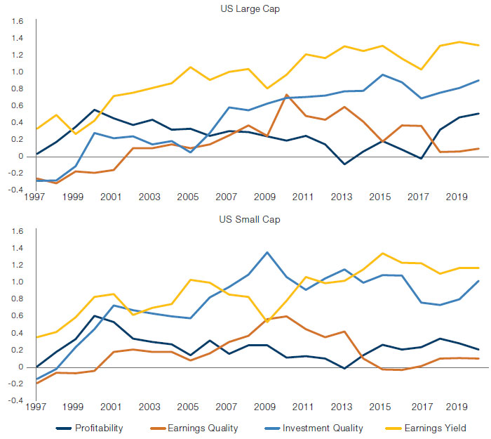
Figure 13 plots the GEMLT exposures of a sector-neutral, long-short decile portfolio of QCI back to 1997. GEMLT Investment Quality, which includes as sub-factors (-) growth in assets, capex and shares, has an almost equivalent expression as Earnings Yield and has been steadily increasing in exposure over the period. As we’ve noted previously, the returns to value and investment quality are correlated. Earnings Quality, which targets the accrual component of quality (mainly changes in current operating assets and liabilities), has dropped in exposure. Profitability, a combination of gross profits to assets and the du Pont ratios of ROE, has a positive expression over the period too, but to a lesser degree than Investment Quality.

Figure 13. Annual Barra GEMLT Exposures for the Numeric Quant Concentration Indicator

Source: 13-F Filing Data, BARRA and Man Numeric Analysis; as of 8 September 2020.

Though it is difficult to quantify directly, we believe that some of the recent decay in most factors must be due to crowding. In Figure 14, we attempt to estimate the marginal impact of crowding on the performance of CMA and RMW. Using monthly return data over a rolling 5-year window (60 months), we regress each factor’s return on the market (‘MKT-RF’), small size (‘SML’), value (‘HML’), CMA or RMW depending on the dependent variable, 12-2 month momentum, residual variance (a proxy for returns to the ‘Flight-to-Safety’ factor), and QCI.

The figure plots the regression, loading (the ‘beta’) on QCI multiplied by the average return of QCI for the trailing five years. For CMA, the independent factor variables largely subsume any power of crowding in explaining returns. RMW, on the other hand, appears to have more sensitivity to crowding over the entire period. We struggle a little with understanding this effect given the relatively low exposure of our crowding factor to profitability. Let’s not overestimate the precision of these figures, but it does appear that crowding has had a recent negative effect that largely offsets prior period benefits, primarily for RMW.

Figure 14. Rolling 5-Year Estimated Alpha Impact from Crowding

Source: Tuck at Dartmouth Kenneth French Data Library; between June 1997 and June 2020.

Conclusion

In this paper, we question whether the assumptions underpinning the ‘bad’ versus ‘good’ growth paradigm of Quality are still valid. It is clear there have been fundamental changes in the competitive and macro environment that have created significant headwinds to quality factor investing, especially within the US.

Contrary to the bad growth thesis, a few companies with network-based business models have been able to effect substantial balance sheet growth while also maintaining high levels of profitability; the market has rightly rewarded these stocks with premium valuations. More generally, the preservation of competitive advantage has become easier over the last 25 years due to superior strategic positioning at the company-level and a favorable regulatory environment.

We cannot completely discount the post-GFC macro environment as an important driver. Whether because of the low-rate environment, the desire for safety, the dearth of other investment opportunities, or merely a facet of the broader growth-value dialectic, it seems investors are willing to pay more for growth than they were previously, and how that growth is achieved doesn’t matter as much as it once did.

What should we do? While the concept of buying higher quality companies retains its intuitive appeal for many investors including ourselves, maintaining conviction in the face of disappointing performance requires an understanding of the underlying causes of performance weakness and potentially some steps to remedy those that are threatened by paradigm shifts in the market. In particular, continuing to evolve one’s definition and implementation of quality has the potential benefits of better risk management, reduced exposure to the deleterious effects of crowding in the more rudimentary quality factors discussed in this paper, and a more nuanced measurement of a company’s true quality above and beyond what is represented solely in its financial statements.

We have to accept that, in the bluntest terms, a significant part of the problem with Quality (and Value) over the last decade is that they have simply been wrong. To some extent, both factors depend on mean reversion (of some combination of growth, profitability, and valuation). The autocorrelation of growth, the stickiness of profitability, and the ever-declining interest rate environment have essentially produced a petri dish of bad Quality (and Value) performance.

These unique circumstances do not, though, guarantee that Quality and Value will be wrong for the next decade, and we know there is some cyclicality to these effects. We do not believe that either factor is irrevocably broken, and it may be that it is just as the last Quality and Value investors are throwing in the towel that the factors finally come back to life. The theory behind these factors still holds, even against the backdrop of a market that appears tailor-made to work against them. We believe the next decade is likely to be substantially more productive for investors willing to keep the faith in the quality and value factors than the past decade was. While we as a firm have gradually become more style agnostic over the past few years and implemented several innovations in our investment process, this does not mean that we have given up all belief in what, we believe, remains a powerful means of thinking about the art of financial analysis.

1. I.e., the more people using a service/product, the more valuable it becomes, a situation that is particularly visible in tech stocks, where widespread uptake confers enduring pricing power and competitive advantage.
2. Facebook, Amazon, Apple, Netflix, Google/Alphabet, and Microsoft. The organisations and/or financial instruments mentioned are for reference purposes only. The content of this material should not be construed as a recommendation for their purchase or sale.
3. See Fama and French, 1993, “Common Risk Factors in the Returns on Stocks and Bonds,” Journal of Financial Economics, and Fama and French, 2014, “A Five-Factor Asset Pricing Model” for a complete description of the factor returns.
4. See Michael J. Cooper & Huseyin Gulen & Michael J. Schill, 2008. “Asset Growth and the Cross-Section of Stock Returns,” Journal of Finance, American Finance Association, vol. 63(4), pages 1609-1651, August.
5. While the CMA factor uses Total Asset growth, a potentially better formulation uses growth in net operating assets = the change in [(Assets – Cash) less (Liabilities – Debt)] scaled by Total Assets which aligns more directly to cash flows (e.g., a rise in accounts payable is cash flow generative). A different methodology for E&I quality in financial stocks could/should be applied as well. We largely ignore these subtleties here by following Fama French’s implementation and excluding financials from our analyses in certain places.
6. Net operating assets are the non-financial assets of the company = (Assets – Cash) less (Liabilities – Debt).
7. Here, we would define optimal size in dollars, where the CEO attempts to maximise profit per unit of capital x total capital, assuming, of course, that per-unit profitability is a declining function of capital.
8. Defined using NBER based Recession Indicators for the United States. Recessions defined as the period following the peak through the trough and vice versa for expansions. Source: Federal Reserve Economic Data.
9. There are whispers of future disruption in antitrust policy, as promulgated by the progressive academics of the ‘New Brandeis School’, who question the benefits of laissez-faire competitive policies. For a discussion, see “The Rise, Fall, and Rebirth of the US Antitrust Movement”; Maurice E. Stucke and Ariel Ezrachi Harvard Busienss Review; December 2017.
10. In our calculation of ROE, we force book value to be the larger of the company’s actual book value and 1% of assets. This ensures that book value is always positive and stabilises ROE estimates for companies with positive earnings but very low book values.
11. Lev, Baruch Itamar and Srivastava, Anup, “Explaining the Recent Failure of Value Investing,” (October 25, 2019). NYU Stern School of Business.
12. Novy-Marx, Robert, 2013. “The other side of value: The gross profitability premium,” Journal of Financial Economics, Elsevier, vol. 108(1), pages 1-28.
13. The industry differences here may not translate directly into portfolio exposures since the variation among companies within each industry may be skewed positively or negatively.
14. Each stock is added to the conglomerate one year after its IPO. One-year ago asset levels are also adjusted at the addition of a new stock such that asset growth is appropriately adjusted.
15. “Are US Industries Becoming More Concentrated?” Gustavo Grullon, Yelena Larkin, Roni Michaely. Review of Finance, Volume 23, Issue 4, July 2019, Pages 697–743.
16. log(0.5)/log(0.63)≈1.5 and log(0.5)/log(0.72)≈2.1
17. This framework may look familiar to those of you who invest in private equity. The decomposition is similar in spirit to Eugene F. Fama & Kenneth R. French (2007) The Anatomy of Value and Growth Stock Returns, Financial Analysts Journal, 63:6, 44-54, DOI: 10.2469/faj.v63.n6.4926.
18. Even with these more robust metrics, we deployed various outlier controls at both the stock and portfolio level.
19. Net buyback yield is calculated as net buyback dollars over the last 12 months, divided by end of period market cap.
20. “On the Importance of Measuring Payout Yield: Implications for Empirical Asset Pricing”; Jacob Boudoukh, Roni Michaely, Matthew Richardson and Michael Roberts; Journal of Finance, 2007, vol. 62, issue 2, 877-915.
21. The composite value consists of an equal weighted combination of Book to Price, Free Cash Flow to Price, EBITDA to Enterprise value, Earnings to Price, Dividend to Price, and Sales to Enterprise Value.
22. Hou, K., Xue, C., & Zhang, L. (2015). Digesting anomalies: an investment approach. Review of Financial Studies, 28(3), 650-705. There is a bit of a factor war afoot with HXZ claiming that FF added CMA and RMW in response to their q-factor model. HXZ also argue the (+) ROE subsumes Carhart price momentum.
23. Because vintages overlap – built monthly and held for a year – the two panels share common return history into May 2010.
24. For (-) asset growth, the 4.9% difference in return due to less multiple expansion is significant at the 5% level, while the level of reduced fundamental growth for (+) ROE of 3.9% is significant at the 1% level. While we argue that they are still economically meaningful, the multiple expansion attribution for (-) asset growth does rise from -4.9% to -3.4% (p-value = 13%), and the total return for (+) ROE shifts from -4.2% to -3.1% (p-value = 15%) if we add a control for recessionary periods. We use Newey-West adjusted standard errors of the coefficients with 5 lags due to overlapping return periods of the vintages when calculating p-values.
25. To unpack this a bit, we can decompose the multiple expansion/contraction into entry and exit multiples. For vintages covering January 1995 to June 2009, the (-) asset growth portfolio traded at an average discount to the market (i.e., the average of Sales-to-EV, GP-to-EV, and EBITDA-to-EV) of 29.0% at entry and 21.6% at exit, implying a benefit from multiple expansion of 7.3% = 29.0% - 21.6% (small discrepancy due to rounding; we see 7.3% in Figure 10). For vintages covering July 2009 to January 2019, the same values are 2.4% multiple expansion benefit = 26.2% entry discount - 23.8% exit discount. Theoretically, then, crowding at entry hurts returns since investors must pay 2.7% more at entry (26.2% - 29.0%) and receive 2.2% less at exit (23.8% - 21.6%) between the two periods of vintages.
26. Hou, Kewei, Chen Xue, and Lu Zhang, 2020, Replicating anomalies, Review of Financial Studies 33, 2019-2133.
27. Chen Xue, Release Notes for June 2020 Update, 16 June 2020.

Hypothetical Results

Hypothetical Results are calculated in hindsight, invariably show positive rates of return, and are subject to various modelling assumptions, statistical variances and interpretational differences. No representation is made as to the reasonableness or accuracy of the calculations or assumptions made or that all assumptions used in achieving the results have been utilized equally or appropriately, or that other assumptions should not have been used or would have been more accurate or representative. Changes in the assumptions would have a material impact on the Hypothetical Results and other statistical information based on the Hypothetical Results.

The Hypothetical Results have other inherent limitations, some of which are described below. They do not involve financial risk or reflect actual trading by an Investment Product, and therefore do not reflect the impact that economic and market factors, including concentration, lack of liquidity or market disruptions, regulatory (including tax) and other conditions then in existence may have on investment decisions for an Investment Product. In addition, the ability to withstand losses or to adhere to a particular trading program in spite of trading losses are material points which can also adversely affect actual trading results. Since trades have not actually been executed, Hypothetical Results may have under or over compensated for the impact, if any, of certain market factors. There are frequently sharp differences between the Hypothetical Results and the actual results of an Investment Product. No assurance can be given that market, economic or other factors may not cause the Investment Manager to make modifications to the strategies over time. There also may be a material difference between the amount of an Investment Product’s assets at any time and the amount of the assets assumed in the Hypothetical Results, which difference may have an impact on the management of an Investment Product. Hypothetical Results should not be relied on, and the results presented in no way reflect skill of the investment manager. A decision to invest in an Investment Product should not be based on the Hypothetical Results.

No representation is made that an Investment Product’s performance would have been the same as the Hypothetical Results had an Investment Product been in existence during such time or that such investment strategy will be maintained substantially the same in the future; the Investment Manager may choose to implement changes to the strategies, make different investments or have an Investment Product invest in other investments not reflected in the Hypothetical Results or vice versa. To the extent there are any material differences between the Investment Manager’s management of an Investment Product and the investment strategy as reflected in the Hypothetical Results, the Hypothetical Results will no longer be as representative, and their illustration value will decrease substantially. No representation is made that an Investment Product will or is likely to achieve its objectives or results comparable to those shown, including the Hypothetical Results, or will make any profit or will be able to avoid incurring substantial losses. Past performance is not indicative of future results and simulated results in no way reflect upon the manager’s skill or ability.