Low Volatility and Interest-Rate Sensitivity

As attention turns to low volatility strategies after a period of market-beating performance, we analyse how skilled managers seek to fully exploit their benefits.

 

Read Article

1. Introduction

As we continue through the tenth year of a record-breaking bull run, talk of recessions and ‘the next crash’ has dominated conversations we have had with institutional investors, who – in many cases – are seeking to de-risk their equity portfolios. 

For some investors, that means reducing equity allocations in favour of other asset classes.

However, for those investors who prefer not to tactically time asset classes or do not want to sacrifice their ability to earn the equity risk premium, low volatility equity strategies (‘low vol’) could be of interest. These are strategies designed to capture equity market returns (or better) with substantially lower downside risk, a topic we have previously discussed in ‘Low Volatility Investing: Topical Concerns’.

There are a variety of considerations for investors when investing in low vol strategies, with the following three being of primary importance: 1) interest-rate exposure and the corresponding relationship between low vol and bonds; 2) crowding due to the popularity of low vol during the past decade in particular; and 3) shorting and how it can help harvest more of the low vol anomaly. 

This article, the first in a three-part series, examines the first of these factors, i.e. the challenges and opportunities that come with the interest-rate exposure of low vol portfolios. 

2. The Link Between Low Vol and Interest Rates

Low vol portfolios tend to be significantly overweight defensive sectors like utilities and consumer staples, a contributing factor to their positive beta to bond returns. Some investors therefore think of low vol strategies as bond proxies that have benefited from declining interest rates over the last few decades. The natural question then becomes: are low vol strategies likely to disappoint in rising-rate environments?

From an empirical perspective, our article ‘Low Volatility Investing: Topical Concerns’ examined the empirics of the rate sensitivity of low vol and found little connection. The lack of a simplistic direct connection between interest rate changes and returns to low vol probably arises from the fact that rate changes are often accompanied by myriad other macro changes, all of which have a variety of implications for low vol. 

From a conceptual perspective, there are at least two possible conflicting explanations of the possible link between bonds and low vol portfolios:

1. Being overweight more stable, profitable, higher yielding names that are often viewed as bond proxies implies higher beta to bond returns for low vol;
2. Theoretically, the shorter duration of typically higher yielding, lower volatility stocks (compared with, say, typical growth stocks) should lead to lower bond beta¹ for low vol.

What do the empirics suggest is going on underneath the bonnet here?

From the late 1960s through to the early 2000s, the equity market had a positive bond beta (Figure 1). Since then, however, equity market returns have been negatively correlated with bond returns (despite both asset classes having positive returns since 2000). In comparison, the beta of a generic low vol portfolio²(illustrated by the dark blue line in Figure 1) has stayed generally positive over the last 40 years.

Figure 1. Beta to 10-Year US Government Bond Returns

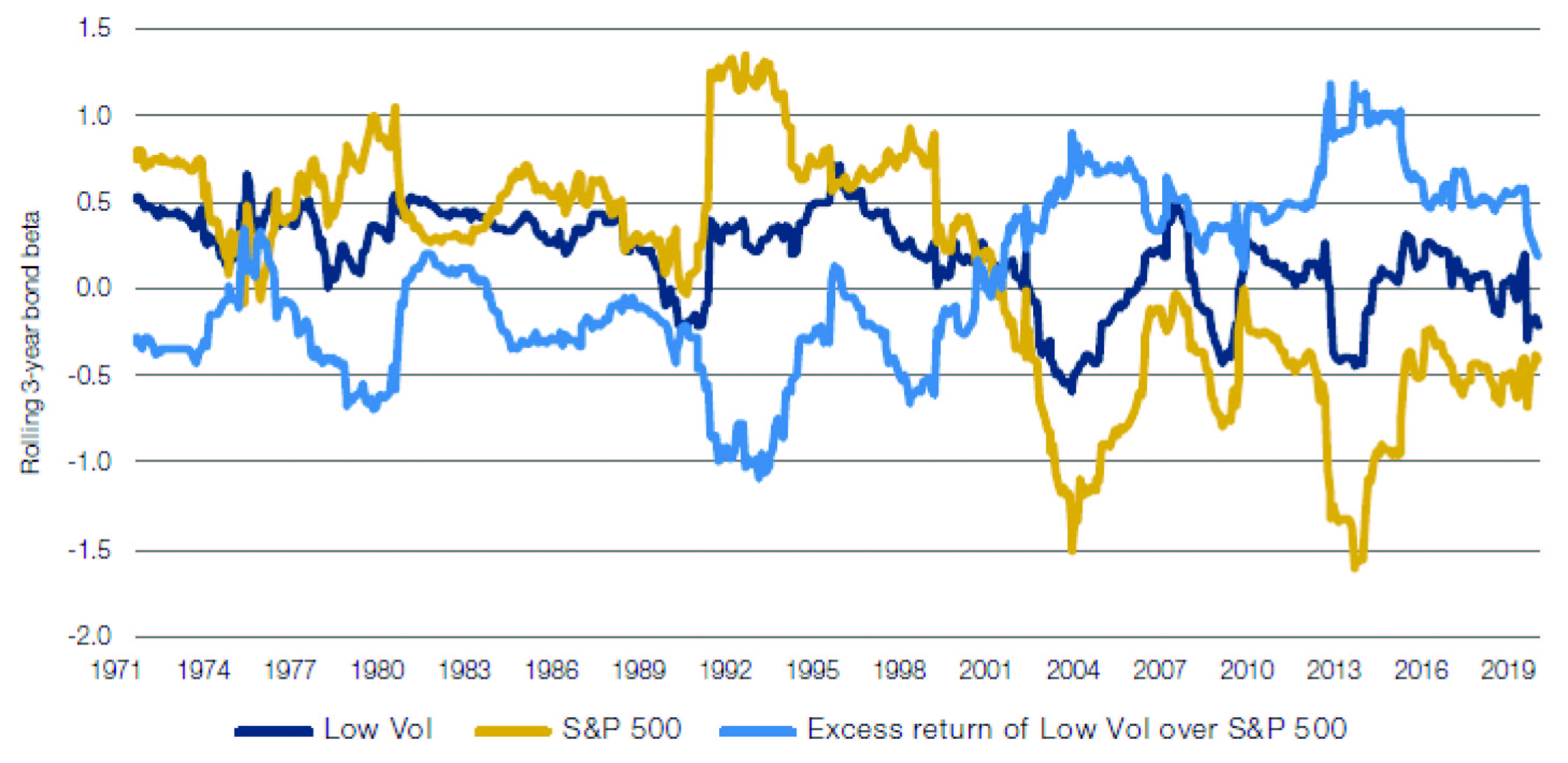
Source: Bloomberg, MSCI, Man Numeric; as of 30 June 2019.

If, as outlined in the first point above, low vol portfolios contain more bond proxy names than a cap-weighted portfolio, then the excess return of low vol can be expected to have a positive bond beta. Empirically, this ‘intuition’ (that a low vol portfolio lies between cap-weighted equities and bonds) is borne out since only about 2000, but not so in earlier periods. As noted previously, this empirical lack of a simple direct connection between low vol and bond returns is probably explained by the fact that rate changes are often accompanied by myriad other macro changes, all of which have implications for the fate of low vol.

Nevertheless, in our view, the fact that low vol strategies have potential interest rate exposure presents investors with either the challenge of neutralising the interest-rate exposure or the opportunity to exploit the exposure in asset allocation.

3. Neutralising the Interest-Rate Exposure

Neutralising the interest-rate exposure can be done in two ways: 

1. The statistical method;
2. The engineering method.

3.1. The Statistical Method

The statistical method involves empirically estimating the bond beta of stocks (similar to how one estimates equity covariances) and constraining this bond beta in the portfolio-construction process i.e. control bond market exposure as a risk factor.

There are two drawbacks to this approach. The first is that beta measurements from a stock-level time series regression have high estimation errors and are sensitive to the look-back window used. There are ways to mitigate the issue by using a Bayesian approach to push a stock’s bond beta toward a sector-average beta, with the assumption that sector- or industry-average bond beta tends to be stable (Figure 2), though no method is perfect.

Figure 2. Sector Average Bond Betas to 10-year US Government Bonds

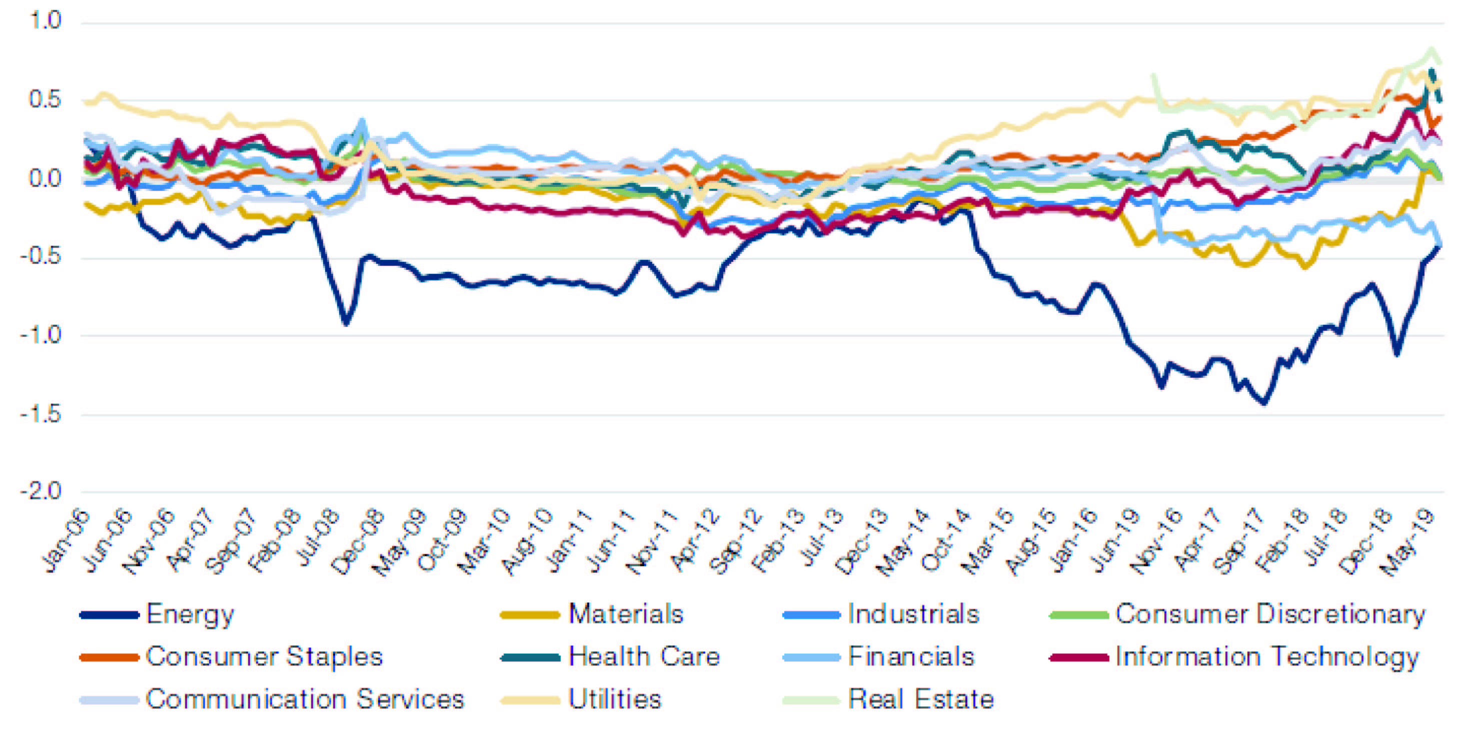
Source: Bloomberg, MSCI, Man Numeric; as of 30 June 2019.

The second – and larger – issue is such statistical approaches typically don’t find that much ex-ante bond beta to be controlled for. Portfolio-level constraints thus have only a moderate impact on the ex-post realised bond beta.

3.2. The Engineering Method

An ‘engineering’ alternative is to nudge the low vol portfolio’s bond beta closer to that of the equity market. This is done through constraints on portfolio exposures that serve as proxies for bond exposure e.g. sector, yield, leverage, etc.

This relies on the assumption that low vol’s bond exposure is generally positive and higher than that of the equity market, which has been the experience for the past 20-plus years. If a low vol portfolio has a positive bond beta, moving it toward the market will decrease the bond beta to be closer to neutral; however, if the low vol portfolio has a negative bond beta (but still higher than the equity market’s bond beta), moving the bond beta closer to market will actually add to the risk by making the bond beta even more negative (Figure 3).

The engineering approach is well suited for a long-only low vol portfolio that is benchmarked to the equity market. In an absolute return, long-short low vol strategy that exploits the anomaly on both the long and short sides to further distance itself from the equity market, the added constraints will be risk additive in the current environment: it tethers the low vol to the equity market, when the equity market itself has a negative beta to bonds.

So, the engineering approach is used if the goal is simply to match the low vol portfolio’s interest rate exposure to that of the equity market.

Figure 3. Shift in Low Vol Portfolio’s Bond Beta When Applying Constraints

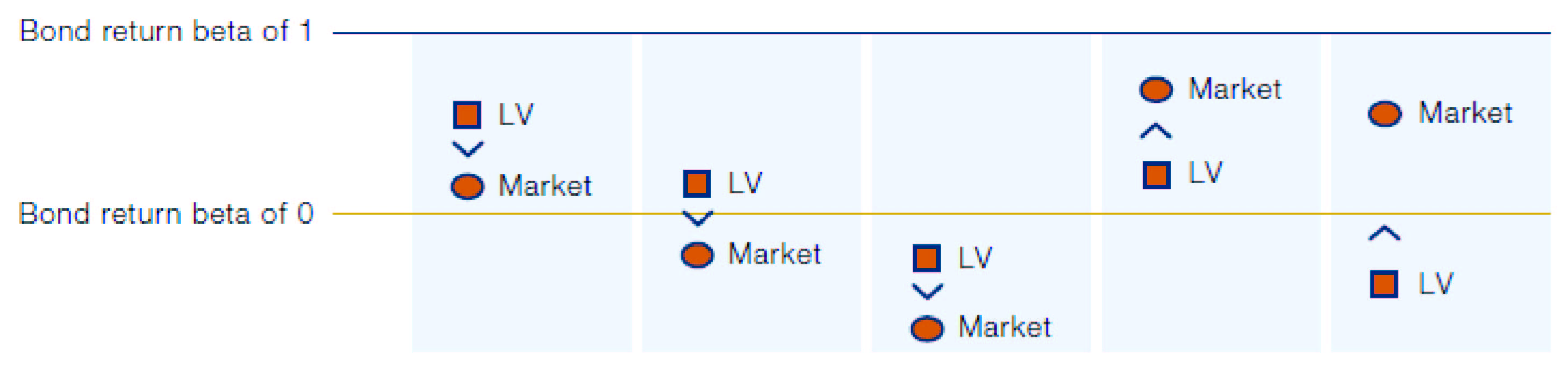
Source: Man Numeric. For illustrative purposes.

However, many investors view interest-rate exposure as an absolute risk. The engineering approach moves the exposure closer to zero only if the exposure of the cap-weighted market lies in that direction; this comes at the price of increased equity beta as any time constraints are added to make a portfolio more like its benchmark, and therefore more like the market, the portfolio’s equity beta increases. For investors who are interested in low vol investing as a diversifying return stream to equities, the increased equity beta may be undesirable. A truly diversifying return stream may well tolerate a positive bond beta, rather than mitigate it by taking on a more positive equity beta.

Empirically, we find that the engineering approach achieved a 10-20% reduction in the realised bond beta (at a cost of higher equity beta). It also reduced the low vol anomaly by about 5-15% of the return attributed to the low vol effect due to the added constraints.³

4. Low Vol in Asset Allocation

The second approach to the interest rate exposure is to embrace the exposure in asset allocation.

Since low vol strategies have comparable performance to the market while maintaining lower drawdowns and risk, it naturally places their return and risk profiles between those of equities and bonds. Can low vol products therefore be considered as an alternative or enhancement to the traditional 60/40 equity/bond asset allocation? For purposes of this example, ‘equity’ is the cap-weighted largest 1,000 US equities and ‘bond’ is the Bloomberg Barclays US Aggregate Index.

In the context of the 60/40 asset allocation, low vol presents two possibilities:

1. As a replacement for the entirety of 60/40, given that low vol itself is seated in between equities and bonds;
2. As a replacement for cap-weighted equities.

4.1: Low Vol as a Replacement for the Entirety of 60/40

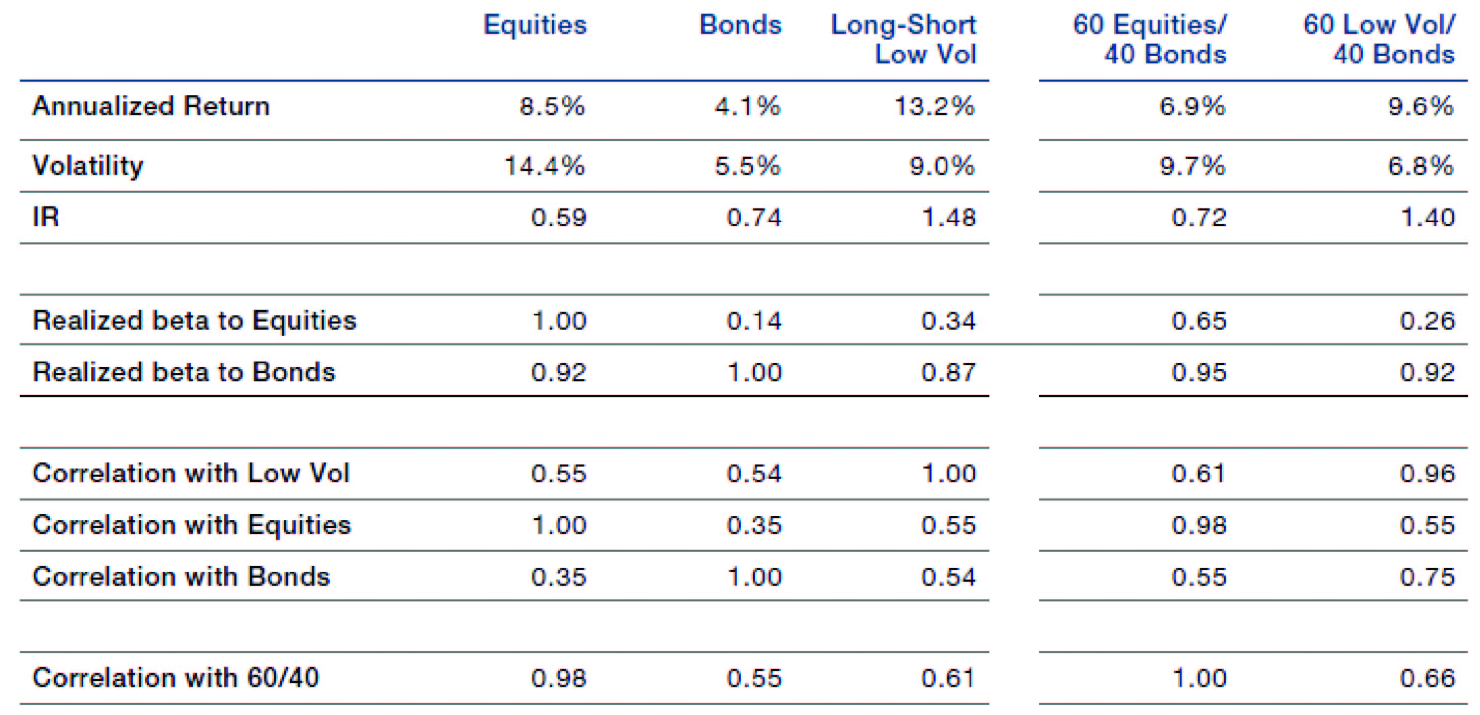
In addressing the first of these, long-history empirics in the US suggest that low vol by itself has a lower information ratio (‘IR’) than the traditional 60/40 approach (Figure 4). It also has consistently worse drawdowns throughout the period (Figure 5).

Figure 4. Characteristics of Equities, Bonds, Low Volatility and Combined 60/40 Portfolios (March 1976 - June 2019)

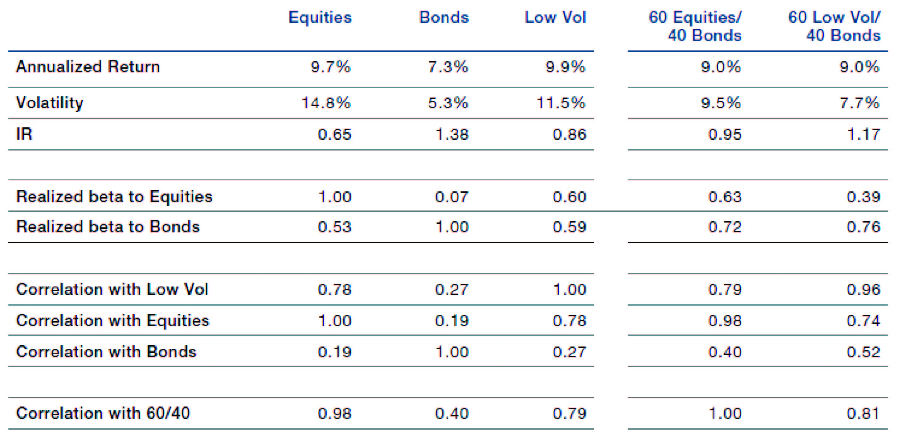
Source: Bloomberg, MSCI, Man Numeric; between March 1976 and June 2019. Equities: Cap-weighted largest 1,000 US equities. Bonds: Bloomberg Barclays US Aggregate Index. Low Vol: Simulated low vol portfolio (US top 1,000 portfolio) after transaction costs. Simulated performance data and hypothetical results are shown for illustrative purposes only, do not reflect actual trading results, have inherent limitations and should not be relied upon.

Figure 5. Drawdowns of 60/40 Equities/Bonds, Low Volatility and 60/40 Low Volatility/Bonds

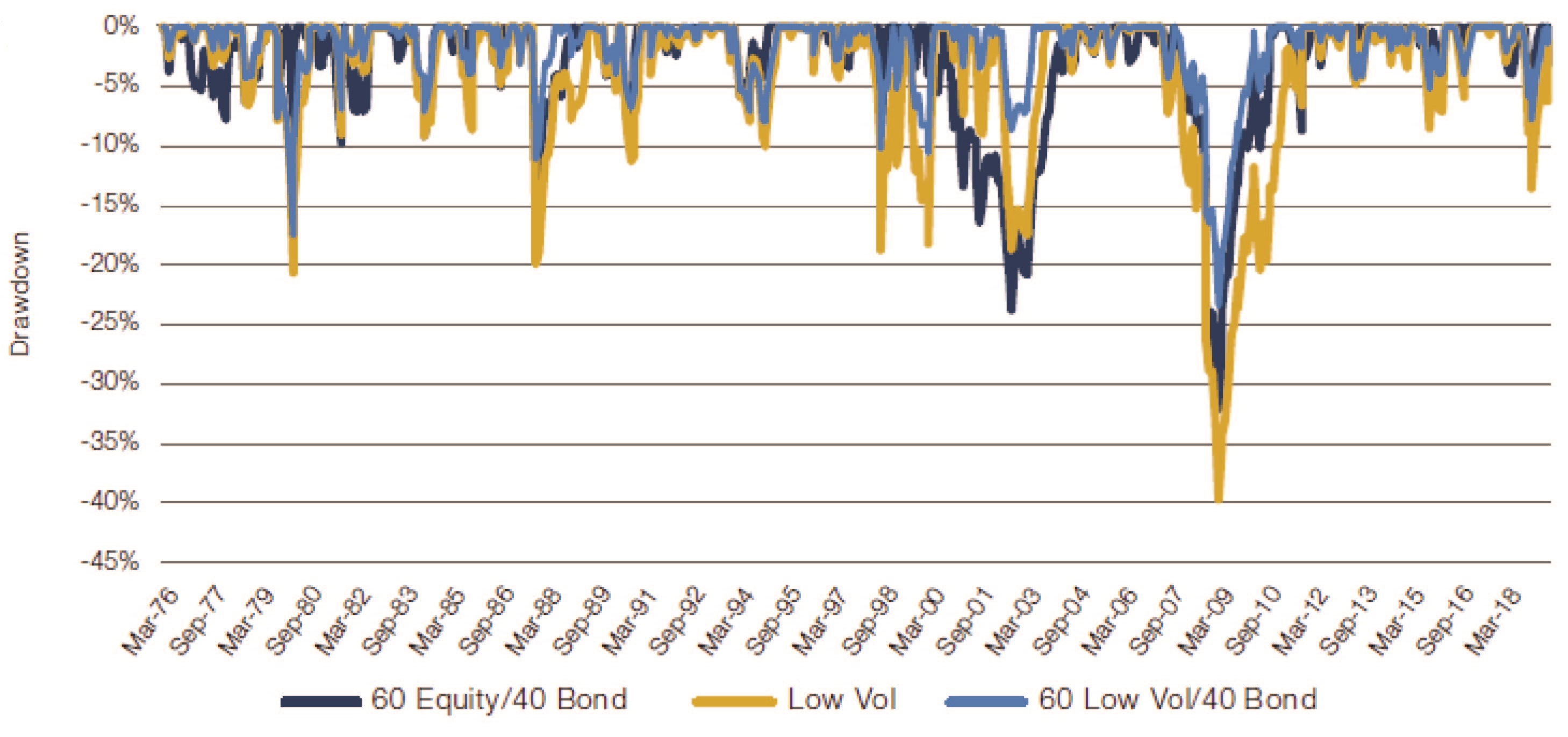
Source: Man Numeric; between March 1976 and June 2019.

So, under what conditions will low vol by itself have a higher IR than 60/40?

The answer is driven by equity and bond performance and the correlations between them. To build this intuition, let’s assume that equity markets return 8% annually at 15% volatility, bond markets return 5% at 5% volatility, and low vol equities produce 8% annually at 11% volatility. At negative equity-bond correlations, the 60/40 approach results in a higher IR than what can be had from low vol by itself (Figure 6).

Correlation between the assets is critical for any asset allocation problem, and the equity-bond correlation has fluctuated over time: it has turned from positive to negative since the late 1990s. Additionally, the greater the IR of equities compared with that of bonds, the greater the attractiveness of low vol as a standalone alternative to 60-40 at any correlation (because the premise of low vol itself, without alpha models and other enhancements, is market-like returns at lower volatility).

Figure 6. Assumed Equity-Bond Correlations Versus Projected IRs

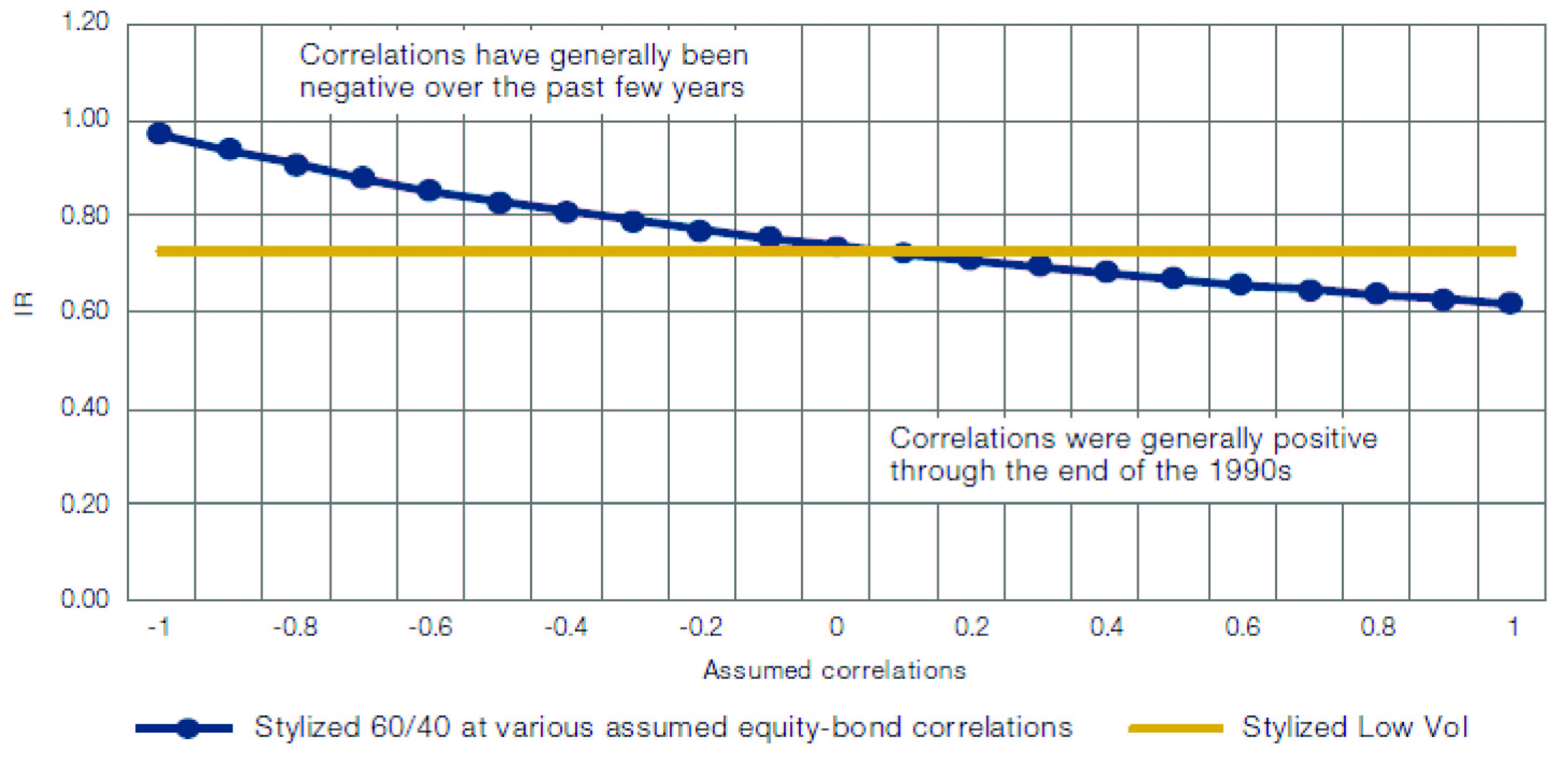
Source: Man Numeric.

Analysis of more recent global data⁴ illustrates that low vol by itself has a superior return and IR than either equities or bonds. Granted, results vary based on regions and timeframes. While low vol dominates 60/40 (Figure 7); in the global context, equities and bonds have had a positive correlation even in the post-2000 time period, which additionally helps low vol. 

Figure 7. Characteristics of Equities, Bonds, Low Volatility, and Combined 60/40 Portfolios (January 2003 - June 2019)

Source: Bloomberg, MSCI, Man Numeric; between January 2003 and June 2019. Equities = MSCI World. Bonds = as in footnote.
Low vol = Long-short low vol over Global top 1000 universe. Simulated performance data and hypothetical results are shown for illustrative purposes only, do not reflect actual trading results, have inherent limitations and should not be relied upon.

4.2. Low Vol as a Replacement for Cap-Weighted Equities

The second possibility is to use low vol as an alternative to the cap-weighted equity index in traditional 60/40 allocations. If low vol (by itself, without any enhancements) delivers ‘market-like returns at lower volatility,’ it will always be a superior alternative to cap-weighted equities in any asset allocation problem.

Substituting low vol for cap-weighted equities, we find that a 60/40 low vol/bonds portfolio returned a similar or higher annual return at lower volatility, over a long history in the US (Figure 4) or a shorter history globally (Figure 7). The superiority held true for most drawdowns historically, where using a 60% low vol allocation tends to deliver lower drawdowns than the 60% cap-weighted equity allocations (Figure 5).

A third possibility is low vol entering the 60/40 asset allocation problem as a separate, third asset class. This is not explored here given that:

1. It is not a different asset, being made up entirely of equities;
2. It has dominated cap-weighted equities empirically (thus allowing cap-weighted equities to enter the solution only under the constraint of requiring high volatility).

5. Summary

Low vol portfolios are expected to have a positive bond beta because they are typically populated with stocks that can be considered bond proxies. Though long-history empirics show no tight connection between excess returns of low vol and change in interest rates, investors would be well-advised to think about this potential exposure, given that much of low vol empirics have been based on a period of falling rates over the past 40 years. In our view, those who see the bond beta as a problem can consider mitigating the exposure, though the price of that mitigation may well be higher equity beta. Those who see it as an opportunity can seek to exploit it by using low vol portfolios in multi-asset solutions.

1. Throughout this paper, bond beta refers to the beta to bond returns (and not beta to rate changes).
2. In this case, a long-short low vol portfolio that is 100% net long by construction. We limit the stocks to be in the top half of the CRSP data universe by cap rank. Net equity beta exposure for this portfolio is generally close to zero.
3. January 2003 to December 2017. MSCI World universe.
4. MSCI World universe and Bloomberg Barclays Global Aggregate; between Jan 2003 and June 2019.

Simulated & Hypothetical Performance

This presentation contains historical simulated and hypothetical performance results for various model portfolios.

Hypothetical Results are calculated in hindsight, invariably show positive rates of return, and are subject to various modelling assumptions, statistical variances and interpretational differences. No representation is made as to the reasonableness or accuracy of the calculations or assumptions made or that all assumptions used in achieving the results have been utilized equally or appropriately, or that other assumptions should not have been used or would have been more accurate or representative. Changes in the assumptions would have a material impact on the Hypothetical Results and other statistical information based on the Hypothetical Results.

The Hypothetical Results have other inherent limitations, some of which are described below. They do not involve financial risk or reflect actual trading by an Investment Product, and therefore do not reflect the impact that economic and market factors, including concentration, lack of liquidity or market disruptions, regulatory (including tax) and other conditions then in existence may have on investment decisions for an Investment Product. In addition, the ability to withstand losses or to adhere to a particular trading program in spite of trading losses are material points which can also adversely affect actual trading results. Since trades have not actually been executed, Hypothetical Results may have under or over compensated for the impact, if any, of certain market factors. There are frequently sharp differences between the Hypothetical Results and the actual results of an Investment Product. No assurance can be given that market, economic or other factors may not cause the Investment Manager to make modifications to the strategies over time. There also may be a material difference between the amount of an Investment Product’s assets at any time and the amount of the assets assumed in the Hypothetical Results, which difference may have an impact on the management of an Investment Product. Hypothetical Results should not be relied on, and the results presented in no way reflect skill of the investment manager. A decision to invest in an Investment Product should not be based on the Hypothetical Results.

No representation is made that an Investment Product’s performance would have been the same as the Hypothetical Results had an Investment Product been in existence during such time or that such investment strategy will be maintained substantially the same in the future; the Investment Manager may choose to implement changes to the strategies, make different investments or have an Investment Product invest in other investments not reflected in the Hypothetical Results or vice versa. To the extent there are any material differences between the Investment Manager’s management of an Investment Product and the investment strategy as reflected in the Hypothetical Results, the Hypothetical Results will no longer be as representative and their illustration value will decrease substantially. No representation is made that an Investment Product will or is likely to achieve its objectives or results comparable to those shown, including the Hypothetical Results, or will make any profit or will be able to avoid incurring substantial losses. Past performance is not indicative of future results and simulated results in no way reflect upon the manger’s skill or ability.