Dealing with Hidden Equity Risk in M&A Deals

1. Introduction

Assets under management in merger arbitrage hedge funds has quadrupled from USD22 billion to USD85 billion in the last 10 years.¹ 2021 was a stellar year for M&A² activity, with more than 40,000 deals announced globally.³ Chances are that a fund manager will, at some point, be exposed to a stock which is the target of an acquisition. As risk arbitrage strategies attract more capital, there is an increased need from risk professionals and hedge fund managers to represent the risk coming from M&A activity as accurately as possible.

However, measuring risk accurately is a challenging task. Indeed, it is a well-known fact that the market price dynamic of equities that are engaged in M&A deals is different to that of the general market, or indeed the historical dynamics of the asset before the deal.⁴ For equities affected by M&A deals, the past dynamics is a particularly poor guide of the expected behaviour in the immediate future.⁵ Therefore, any methodology which uses the past as a predictor of the future is almost certain to misrepresent the risks without adjusting for this limitation.

The goal of this article is to:

• Discuss the price dynamics around M&A deals;
• Discuss how to measure M&A risks and the limitations of the different measures;
• Present a hypothetical risk model which corrects for the Value-at-Risk (‘VaR’) limitation.

2. Price Dynamics Before and After M&A Deal Announcements

Consider the proposed acquisition by a stock A (acquirer) of another stock T (target). For the purpose of this paper, we use an actual deal, which was announced on 24 May 2021 and was terminated on 26 July 2021.

Figure 1 shows the share prices of the both the acquirer and the target companies. The vertical black lines on the chart indicate when the deal was announced, and subsequently terminated.

The figure shows a typical evolution of events for a cash deal. When the deal is announced, there are jumps – ups and down – in both companies’ share prices. Following the announcement, the target tends to trade with reduced volatility centred around a price that reflects the value of the cash deal and the market’s expectation of the deal completing. Finally, there are further jumps when the deal terminates or completes as the new information enters market expectations.

Figure 1. Share Prices of Acquirer and Target

Problems loading this infographic? - Please click here

Source: Man Group; as of September 2021. Past performance is not indicative of future results.

3. Methods of Measuring M&A Risk

There are various accepted market practices to adjust for change in market behaviour resulting from M&A deals. Below are some examples of risk adjustments applied by practitioners.

3.1. Equity Exposure

The traditional measure of equity risk in a fund is the equity exposure which measures the percentage of a fund’s net asset value (‘NAV’) allocated on a long or short equity position in market value terms. However, for an M&A deal, practitioners can sometimes adjust the equity exposure by assuming that all M&A deals successfully complete. For example, in the case of an all-cash transaction, the M&A-adjusted equity exposure is equal to zero, while in the case of all-stock transactions, the M&A-adjusted equity exposure depends on the number of shares of the acquiring company that will be obtained at the end of the deal. In the case of a mixed deal, a combination of both approaches can be taken.

3.2. M&A Deal Break Cost

Unfortunately, the equity exposure metric described above does not capture the P&L impact if the deal does not go through. Therefore, to measure the downside P&L impact, an additional risk metric often used by M&A fund risk departments – the ‘deal break cost’ – is computed. It attempts to calculate how much P&L would be lost if the deal does not go through. This is calculated by assessing the levels at which the acquirer and the target companies would trade if the deal falls apart and derive the resulting P&L.⁶

3.3. VaR

While the adjustments described above can be effective for static risk measures, they must be augmented for statistical⁷ measures by considering the possibility that the deal breaks.

There are different types of VaR models used to quantify the tail risk of a fund (see the appendix for additional details about the different methodologies). The different VaR models generally operate, directly or indirectly, on recent history to construct a distribution of scenarios that are possible in the immediate future.

3.4. M&A VaR Limitations

Unfortunately, none of the widely accepted models adequately capture M&A deal behaviour. For example, we look at the case of an M&A cash offer on a target company. In this case, there are two possible outcomes for the target company:

• Case 1: The deal goes through and the cash is paid to the shareholders;
• Case 2: The deal does not go through (deal break event) and the stock price of the target drops.

It is easy to be convinced that after a deal announcement, the payoff of holding the target company is similar to the payoff of a zero-coupon bond. Indeed, a zero-coupon bond also has two possible outcomes at maturity:

• Case 1: The bond does not default and pays par to the bondholders;
• Case 2: The bond defaults (i.e. a default event occurs) and the bond price drops.

Figure 2 shows the 6-month (i.e. 131-day) rolling volatility in the target. In normal market conditions, the rolling volatility gives a reasonable estimate of forward-looking volatility. In this case, however, it is less useful as an estimate since the short-term volatility once the deal is announced reduces, and the 131-day rolling volatility remains high due to being heavily influenced by the period before the deal announcement. It slowly decays after the deal announcement, but still remains a significant overestimate of the volatility over the deal period.

Figure 2. Six-Month Rolling Volatility of Target Company

Problems loading this infographic? - Please click here

Source: Bloomberg; as of September 2021.

Figure 3 illustrates how the sudden change in price activity during the deal period has a large impact on VaR (plotted in blue). The daily P&L resulting from holding the target stock is plotted in grey. The VaR is supposed to capture the tail risk of holding the target stock, and one would reasonably expect some grey bars to negatively cross the blue line. This is clearly the case before the announcement is made. However, after announcement date, the VaR seems to overstate the tail risk (i.e., none of the daily P&L grey bars negatively cross the VaR).

Figure 3. Target Company’s Returns and VaR

Problems loading this infographic? - Please click here

Source: Bloomberg; as of September 2021. Past performance is not indicative of future results.

Also shown in the figure is the expected ‘deal break cost’ (in yellow) between when the deal was announced and the deal was terminated. The resulting quantification materially reduces the expected risk. While the VaR was never breached, the ‘deal break cost’ metric shows a level of risk which is beached four times in the period, suggesting that the order of magnitude of the risk is more adequate. This is why we believe it should be the preferred metric as the primary model input of VaR during the period of the deal.

4. Addressing VaR Limitations

4.1. Modelling

One way to deal with overstating the tail risk is to choose an M&A diffusion model which is inspired by multi-asset credit default pricing models. In the credit models, the events are the defaults. The same mathematics¹⁰ could be applied to give a realistic model of M&A deal break events. In the case of M&A deals, the events are the deals breaking.

To do this, the average percentage of a deal breaking as well as the average length of the time it takes for a deal to go through needs to be calculated.

4.2. Assumptions

The assumptions used are:

• The M&A deal breaks are independent from each other and from the market dynamics. We assume that a given M&A completion does not have an impact on another M&A deal completion. This is not always an accurate assumption as there are times when financing conditions worsen. As such, M&A deals are likely to either all complete or for none of them to complete (i.e., there is a correlation and the deal completion events are not independent);
• The probability of deal break is calibrated to 6% over a 109-day period.¹¹

These two assumptions are based on historical M&A deals (please see Section 4.3 for more details).

• The financial impact of the deal break is taken from a hypothetical ‘deal break cost’ model. As mentioned above, the ‘deal break cost’ measures the P&L impact of a deal breaking. This is an important input to the model since estimates of a deal breaking is based on the two assumptions above. Furthermore, for estimations on an M&A deal breaking, the P&L impact is given by the deal break cost;
• The deal break and market risk distributions are combined to create a single distribution, which is then used to calculate the VaR. This step is standard. From the P&L, the tail is calculated using a given quantile.

4.3. Calibration of the New Model

The assumptions above are based on an analysis of more than 15,000 M&A deals between 2010 and 2021. Each deal could also have many revisions as new acquirers and targets enter and exit the scene and there can be fierce competition between bidders too.

Figure 4 shows the number of deals in a sequence of increasing duration buckets. It shows, for each day after the deal announcement, the number of deals which completed (in yellow), and the number of deals which broke (in blue). The simplest results from this data are:

• An average of 6% of deals break;
• The average deal length is ~109 days;
• Most deals are completed relatively quickly, but there a small number of deals that take more than a year to complete.

Figure 4. Histogram of Average M&A Deal Length and % of Deals That Break

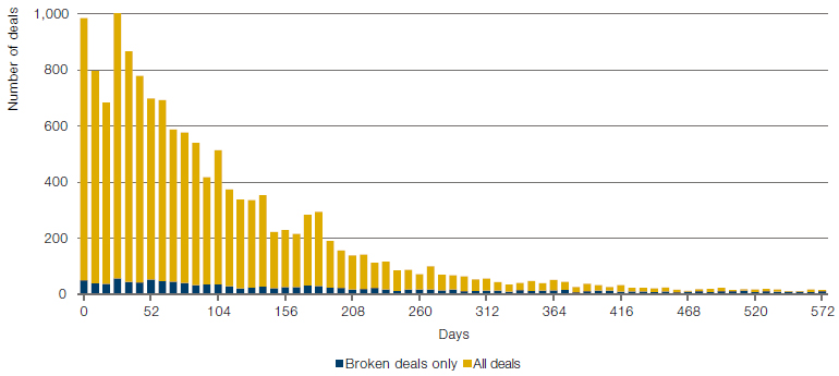
Source: Man GLG; between 2010 and 2021.

The traditional VaR measures overstate M&A risk arbitrage exposures. However, when using a VaR model inspired from the credit models (which replaces default events with deal break events), one gets a result which is more in line with what can be realistically expected. This approach captures the probability of deals breaking along with their own deal break cost payoffs in those events.

5. Conclusion

There are many subtleties to consider when measuring risk coming from M&A deals in a portfolio. On one hand, expected volatility is complicated to assess in M&A deals post the deal announcement. On the other hand, capturing the right level of tail risk is critical when it comes to quantifying the VaR. In any case, whichever approach is taken, capturing adequately the risk coming from M&A deals is a critical aspect of risk management which, in our opinion, requires specific adjustments, some of which are judgment based.

6. Appendix

6.1. VaR Methodology

6.1.1. Parametric VaR

The parametric approach assumes the returns of the funds are normal. The calibration of the returns will define the volatility to use in the model. The advantage of the model is that the results are extremely easy to calculate via a closed form solution.¹² Therefore, the VaR can be calculated with most parameters easily for all quantiles and all horizons. The limitation of this approach is that empirical returns are non-normal^13,14 and therefore the VaR is off, especially for the tail of the distribution at 99%.

6.1.2. Historical VaR

The historical VaR model takes current positions and simulates the fund P&L in a given lookback period. It then calculates the tail risk at a given quantile. This approach is powerful because it is very intuitive: it quantifies the tail when keeping the position unchanged during the lookback period. It also captures, to some extent, the fat tail that markets exhibit. The limitation of this approach is that it isn’t as stable as one could hope for simplistic quantile calculation.¹⁵ Another potential issue is that one can’t shock the volatility or correlations easily with this methodology (which the parametric approach allows for).

6.1.3. Monte Carlo

The Monte Carlo metric takes the current position as an input to the model and simulates the hypothetical P&L of the fund in the future for a pre-set horizon. To simulate the future P&L, a market calibration, usually performed at asset level, is made. This calibration is complicated and attempts to quantify the volatility and the correlation structure between assets. Once done, thousands of paths can be simulated and a quantile taken. The advantage of this approach is that it can capture some form of tails because: 1) it calibrates on historical return; and 2) the diffusion process is decided by the model developer and therefore can be non-gaussian.¹⁶ Another advantage is that the methodology can calculate the VaR assuming a different volatility than the observed one or can update the correlation structure. The main issue with this approach is that it is complicated and costly to calculate.

6.2. Controlling the Quality of the Results

A couple of important checks need to be performed to ensure the VaR model is adequate and fit for purpose. There are two back-testing tests which can be performed: the Binomial test and the Mixed Kupiec test.¹⁷

The Binomial test is a straightforward test to compare the expected number against observed number of VaR breaches. Under the null hypothesis, the predicted VaR numbers are accurate and the number of VaR breaches follows a binomial distribution, from which the p-value of standard test statistic can be calculated.

The Mixed Kupiec test is useful in studying the independence of VaR breaches by considering the lengths between consecutive breaches. This test is very sensitive to multiple VaR breaches that occurred in a short timeframe.

Particular attention needs to be given to analysing the P&L versus the VaR upon a deal breaking to assess whether the VaR is too high or too low.

1. https://www.barclayhedge.com/solutions/assets-under-management/hedge-fund-assets-under-management/merger-arbitrage/
2. Merger and Acquisition
3. Source: Bloomberg.
4. Characteristics of Risk and Return in Risk Arbitrage, The Journal of Finance, Mark Mitchell and Todd Pulvino, Dec 2001
5. For example, M&A practitioners are aware of a change in expected volatility before and after deal announcement dates.
6. This is a particularly complicated task because it does require a judgment on where market trades if the deal fails which itself depends on funds positioning which isn’t known.
7. Statistical measures are risk measures which use a distribution of outcomes to measure properties such as standard deviation or VaR (tail risk).
8. It is always true that ‘Past Performance Is No Guarantee of Future Results’ however what we are saying here is slightly different. In general, for a Risk Arbitrage deal, we know for certain, that past price action before announcement date is not a good representation of future price action i.e., after announcement date.
9. The tail risk of an M&A deal is related to the deal break cost.
10. Using independent Poisson processes:
https://en.wikipedia.org/wiki/Poisson_distribution
11. See sections 4.3.
12. A mathematical expression expressed using a finite number of standard operations.
13. Empirical Distributions of Stock Returns: Scandinavian Securities Markets, 1990-1995, Felipe Aparicio and Javier Estrada.
14. The variation of Certain Speculative Prices, Benoit Mandelbrot, The Journal of Business, Vol. 36, No. 4 (Oct 1963), pp. 394-419.
15. The output from the VaR model is strongly dependent on the modelling of the quantile and how it is extrapolated from the data.
16. This method enables the user to use a distribution which exhibit fat tails, which gaussian distributions do not have and can be therefore be a problem.
17. https://www.mathworks.com/help/risk/overview-of-var-backtesting.html