Portable Alpha: Ask the Hard Questions

Introduction

Interest in portable alpha strategies is surging. The potential double advantage of more efficient capital use, combined with a wider choice of alpha sources, appears to be driving this. We have covered the fundamental concept of portable alpha here¹ but in its simplest terms, it involves replacing the physical equity (or other benchmark) exposure (beta) with derivatives to free up cash, then deploying this into an uncorrelated return stream (alpha).

Yet this does not automatically equate to success. The quality of the alpha, the structure, liquidity, fees and rebalancing are details rarely addressed in introductory material. It is straightforward to build a portable alpha structure that works in benign conditions, but how do we build one that can withstand a liquidity shock or sudden spike in market volatility?

In this paper, we move beyond the introductory definitions and ask the hard questions. We examine how much cash to hold to avoid being closed out, how liquidity in alpha affects suggested cash buffers, and the rebalancing trade-off between closely replicating the beta versus maintaining a more constant one-to-one weight between alpha and beta. There are further considerations too: are investors being charged for the structure beyond their manager’s alpha fee? And is the structure optimal or does it risk cross contamination with other investors?

The hard questions

1. Cash buffers and correlations – is there enough spare cash in the structure to survive a major shock?

It is tempting to run a minimal level of cash in the beta component of a portable alpha structure. If an S&P 500 investment can be funded with just 10% cash, why not deploy the remaining 90% into alpha exposure for higher return opportunities? This logic holds in normal times, but not when a shock hits.

Liquidity management was a major contributor to the failure of portable alpha in 2008. As markets sold off, investors faced margin calls in their beta allocations. In October 2008, the S&P 500 shed 16.8% in a single month: those without reasonable cash buffers either had to find liquidity in their alpha (many were not liquid, and were unable to generate cash within a month timeframe), or were forced to close out their beta position. This loss of market exposure may be a serious outcome, locking in losses with reduced prospects of participating in the eventual recovery.

Most portable alpha structures today have larger buffers than those seen in 2008, though we believe many remain insufficient. The key question is whether there is enough cash to survive a shock without resorting to hurried sales of either beta or alpha exposure. One useful way to model this is to take the largest ever rolling monthly losses for the S&P 500 and assume a rebalancing of alpha and beta at each month end. In Figure 1, we show the cash level in the structure, based on a beta of S&P 500 and a hedge fund alpha (SG Trend Index, used for illustration) weighted one-to-one and rebalanced monthly.

Figure 1. Portable alpha unencumbered cash balance, assuming cash is used in the following ways: the alpha strategy 60%, the beta (S&P 500) 40%. The 40% is comprised: initial margin 10%, initial unencumbered cash 30%

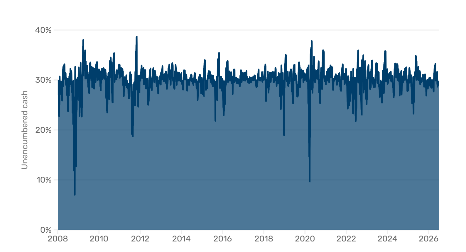
Shows unencumbered cash through time assuming monthly rebalancing between alpha and beta. Alpha illustrated by SG Trend index, beta by S&P 500 Index. Date range: January 2008 to March 2026. Source: Man Group database, SocGen.

As expected, the ‘spare cash’ settles around 30%, which is the target in Figure 1 above. However, it shows some major deviations around market shocks. In October 2008, for example, unencumbered cash fell to 7%. Anyone running a ‘safe’ cash buffer of 20% would have been in serious trouble, facing margin calls they potentially could not meet. The same applied in March 2020.

Once this cash buffer is exhausted, investors are in a tough spot. One option is to deleverage the alpha to raise cash, but this creates problems of its own: the alpha may not be liquid enough to sell down in a crisis, or the monthly or quarterly redemption window may have already passed. Selling the beta, as mentioned, means potentially missing a market recovery, and reestablishing the position requires either an additional capital contribution, or waiting until the next alpha dealing period.

Consider an investor forced to sell near the lows of March 2009. The S&P 500 closed at 676 (price index) on 9 March 2009, its trough for the cycle. Even assuming a short notice period and month-end dealing to sell some alpha, the earliest realistic re-entry point for the beta was the following month end on 31 March (798), by which point the index had already rallied roughly 18%. An investor unable to deal until the following month on 30 April 2009 (873) would have missed a rally of around 29%. The forced seller therefore risks crystallising losses near the bottom and forgoing a significant portion of the rebound. This is precisely why the liquidity of the alpha and the size of the cash buffer are so critical.

Based on our modelling, 30% appears to be a prudent margin of safety for monthly-dealt alpha (for the avoidance of doubt, this 30% unencumbered cash is held in addition to the 10% already used for initial margin, bringing the total cash supporting the beta to 40%). For quarterly-dealt alpha, the longer redemption cycle means 40% unencumbered is more appropriate. Where the structure cannot hold this much unencumbered cash, a committed credit facility or access to callable capital may be appropriate as a backstop to meet margin calls.

The above analysis assumes the alpha component displays no correlation with the selected beta source, and importantly that this lack of correlation persists even during tail events. The latter assumption caused significant problems for portable alpha strategies during the Global Financial Crisis (GFC), when a spike in correlations meant that alpha sources, intended to be diversifying, compounded losses in the beta component. Those lessons should have been learned by today’s providers, but it is important to verify that. A practical approach is to request the return stream of the alpha source and examine its long-term correlation to the beta index, both across the full distribution (using all the data) and in the tails (using, for example, only the worst 10% of returns for the beta index). Any structural correlation here is a red flag warranting further investigation.

The bottom line: We believe at least 30% unencumbered cash is appropriate for monthly dealing strategies, and more for quarterly or less liquid strategies. Also check the correlations in the tails.

2. Fees – is the manager only charging for alpha?

Delivering portable alpha requires two capabilities. First, a high-quality alpha source, preferably with a track record of at least five years. This is the value add, and where we think fees are justified. Second, the structuring capability to manage the separate alpha and beta components. This includes accessing the beta via swaps or futures and managing the associated risks and cash flows.

The structuring component is an operational service. Accessing S&P 500 exposure via a total return swap or futures is straightforward for any institutional-grade asset manager and the cost is simply the spread charged by the counterparty bank. It is therefore reasonable to ask whether any fees beyond the alpha management fee reflect genuine additional expertise. A manager with strong alpha and structuring expertise will typically not charge any additional management fees for the service of setting up the structure. There may be legitimate reasons for using an intermediary (for example, access to a capacity-constrained alpha source) but investors should be especially vigilant about total fees charged for operational services and access to third-party alphas.

Why does this matter? Figure 2 illustrates the total compound return of a US$100 million investment in a portable alpha structure. Structure A earns 7% per annum from the beta component and an additional 5% per annum from the alpha component before fees, for a total of 12%. The fee is a flat 1% on alpha. Structure B earns the same returns but also charges a 0.5% ‘structuring fee’ on top of the 1% on alpha.

Figure 2. Identical portable alpha structures, except structure B charges an additional 0.5% ‘structuring fee’

Problems loading this infographic? - Please click here

Illustrative example to show effects of fee compounding over time. Investment size and return rate are purely hypothetical and not indicative of any current or future investments.

For a long-term investor, the difference is stark. The additional 0.5% charge for the structuring and beta, compounded over 25 years amounts to US$150 million in lost returns, more than the initial investment. It pays to ask the hard questions about fees and whether charges extend beyond the alpha.

The bottom line: Consider whether fees are being charged on anything other than the alpha.

3. Rebalancing – how often, if ever, should I rebalance my alpha and beta?

It is tempting to think about portable alpha as simply "index return + alpha return". In reality, the moment an investor or manager rebalances the weights (e.g., selling alpha to buy more beta after a dip, or simply following a quarterly rebalancing rule), the portfolio no longer perfectly replicates the index. It becomes an actively traded position.

This can be remedied by buying alpha and beta on day one and never rebalancing. This would deliver the index return, plus the alpha return (less some financing costs on both sides). In practice, however, few investors (including ourselves) would do this. First, maintaining a good balance of alpha and beta is important. Once the ratio drifts from one-to-one, investors lose clarity on their underlying alpha-to-beta exposures and their ability to manage allocations accordingly. A second consideration is investor flows. Without rebalancing, the alpha-to-beta mix can drift indefinitely from its target. Third, rebalancing helps mitigate the risk of depleting the cash buffer and ensures the portable alpha structure maintains its long term liquidity and diversification targets.

So what is a sensible rebalancing approach? Most common is calendar-based rebalancing on a fixed schedule, say monthly, quarterly or annually. An alternative is threshold-based rebalancing, triggered only when the alpha-to-beta mix drifts beyond an agreed tolerance, such as +/- 10%. A third option combines both, for example an annual rebalance with a 10% tolerance. In Figure 3, we consider a simple annual rebalance.

Figure 3. Portable alpha portfolio exposure of S&P 500 and SG Trend with annual rebalancing

Problems loading this infographic? - Please click here

Shows exposure by asset as a percentage of NAV over time. Rebalances annually on the first business day of the year. Uses target weights of 100% S&P 500 and 100% SG Trend. Date range: January 2000 to March 2026. Source: Man Group database.

As shown, the structure goes through periods with the beta above or below 100%. How does this impact performance versus other frequencies? This is visualised in Figure 4, which compares three-year rolling returns across different rebalancing rules (monthly, quarterly, threshold-based) against an annually rebalanced baseline.

Figure 4. Three-year rolling returns (annualised) of different rebalance frequencies over a yearly rebalanced portable alpha

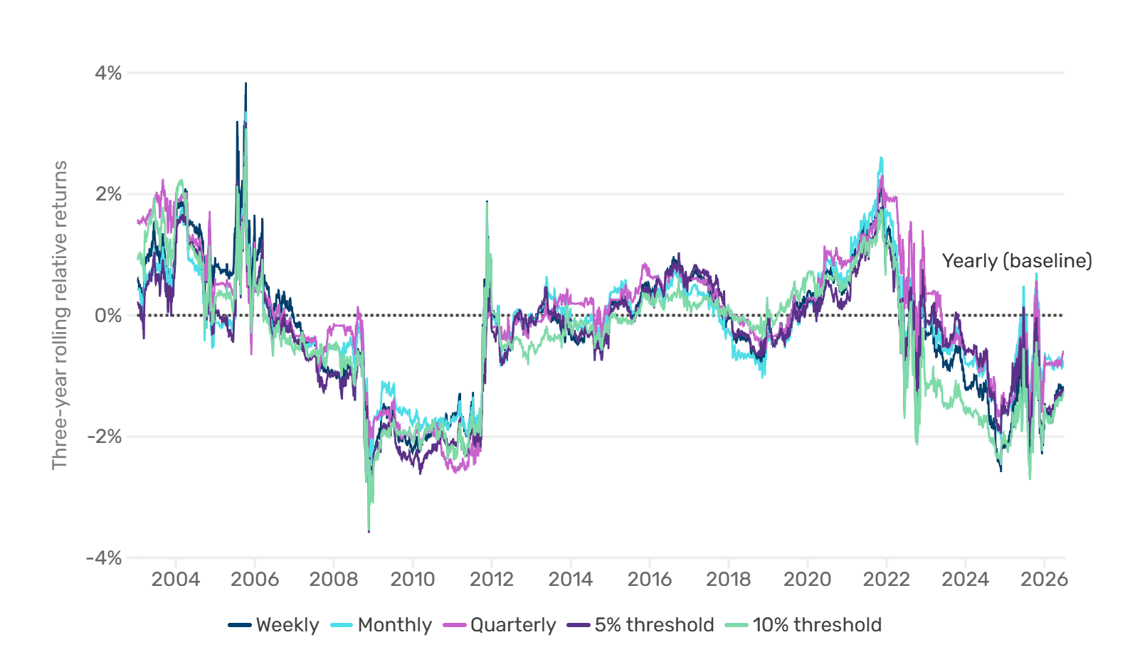
Past performance is not indicative of future results. Shows excess return versus a yearly rebalanced baseline for differing frequencies and threshold-based rebalance models. Uses target weights of 100% S&P 500 and 100% SG Trend. Indices are unmanaged. Performance for the S&P 500 is shown gross of fees while the SG Trend is net of underlying manager fees. One cannot invest directly in an index. Date range: January 2003 to March 2026. Source: Man Group database.

In most periods, the rebalancing frequency has no material impact on returns. However, when both the alpha and beta components experience volatility simultaneously, it can have a notable impact. The GFC is a case in point: a positively performing alpha combined with sharply falling equity markets meant that more frequent rebalancing reinvested alpha gains into a still-falling equity market, compounding losses. Annual rebalancing avoided this as alpha gains were not moved into the beta until year end. The impact is illustrated in Figure 5.

Figure 5. Cumulative return of different rebalance frequencies over a yearly rebalanced portable alpha portfolio (2008-2010)

Problems loading this infographic? - Please click here

Hypothetical returns are not indicative of future results. Shows excess return versus a yearly rebalanced baseline for differing frequencies and threshold based rebalance models. Uses target weights of 100% S&P 500 and 100% SG Trend. Indices are unmanaged. Performance for the S&P 500 is shown gross of fees while the SG Trend is net of underlying manager fees. One cannot invest directly in an index. Date range: January 2008 to December 2009. Source: Man Group database

In summary, the performance differential between rebalancing approaches is expected to be small over the long run, but can be material in periods when alpha and beta diverge sharply. While an index manager rebalances frequently to reduce tracking error, doing so between portable alpha sleeves actually introduces tracking error by disrupting the compounding of the underlying market exposure. Therefore, less frequent rebalancing (for example, annually) better replicates the returns of the underlying beta index. This is often the primary objective for investors replacing a passive allocation.

On the other hand, regular rebalancing preserves the intended diversification of the structure and simplifies cash flow management. Perhaps the best of both worlds is a slow calendar rebalance (e.g. yearly) combined with a threshold to ensure the alpha-to-beta mix never drifts too far. Investors would be wise to discuss the rebalancing rule before allocating, as well as stress-testing the structure against historical scenarios such as 2008 to understand how it would have behaved.

The bottom line: It’s often a surprise to investors that once a portfolio is rebalanced, it no longer replicates the original beta index it was trying to beat. A less frequent rebalancing schedule could help address this, and combining it with a tolerance-based approach could support the portfolio's intended liquidity and diversification characteristics.

4. Structures offered to investors: share class or dedicated structure?

A common approach is to offer portable alpha as a share class of an existing commingled fund. This is operationally simple but brings risks, such as margin calls on the beta exposure, into a fund where existing investors may not have signed up for them. A dedicated vehicle may help to mitigate some of these risks.

For dedicated structures, there are several routes. A standalone vehicle suits investors with sufficient scale, though the costs and infrastructure burden can weigh on smaller allocations. Another option is a segregated portfolio structure, where multiple segregated portfolios (SPs) sit within one legal entity, each ring-fenced from the others. Entity-level costs are shared, lowering the burden per investor and making the structure viable across a wider range of allocation sizes. As more investors are onboarded, those shared costs spread further, bringing down the burden over time.

One approach is to group SPs by beta, so all investors within a given SP share the same underlying index exposure. This keeps margin dynamics consistent across the SP and avoids mixing investors with different beta risk drivers. Where specific requirements demand it, dedicated SPs can still be carved out.

Even within such a structure, it is worth asking about residual risk. If one SP cannot meet its margin calls, could that create problems for others on the platform? With vanilla and liquid beta instruments, sensible cash buffers (see question one), and active monitoring at the SP level, we believe this risk is manageable. It is likely also materially lower than the cross-contamination risk inherent in a shared share class structure.

Of course, the segregated portfolio route is more operationally complex and typically requires a longer lead time to set up. A share class on an existing fund may therefore be preferable for smaller allocations, or even as an interim step while a more comprehensive platform is developed.

The bottom line: A dedicated structure may reduce cross-contamination risk and is more scalable, though this typically comes at the cost of a longer set up time.

5. Futures or swaps – which instrument should I select for my beta?

A common question we hear from investors is whether to use equity index futures or total return swaps for their beta exposure. The short answer: we believe it doesn't matter too much. Both give leveraged exposure to the index and, over time, the returns are near identical. The law of one price/no arbitrage ensures this as if one becomes meaningfully cheaper than the other, arbitrageurs close the gap.

So what are the key considerations?

Leverage: With a swap, the cost of leverage is explicit as investors pay a benchmark rate (SOFR) plus a spread, agreed upfront in the term sheet. With futures, the cost is implicit, baked into the futures price via the cost of carry relationship. Either way, investors pay for leverage.

Margin: Where it matters more is margin. Swap initial margin is typically fixed (around 10% to 20% of notional) and predictable. Futures margin is set by the exchange and moves with volatility. Historically, it has only exceeded 10% a handful of times, including during the GFC and the COVID pandemic, but that variability is worth noting.

Choice: Swaps offer a wider choice of beta. Liquid equity index futures exist for perhaps 30-40 indices globally so for a benchmark like the S&P 500, that's fine. But for a hedged implementation, a regional index, or more bespoke indices, swaps are likely the more practical route. They also deliver the total return of the index by contract, whereas futures require quarterly rolls that can introduce small sources of tracking error.

Counterparty risk: Futures have the edge here. Centrally cleared, removing bilateral counterparty risk, and requiring no ISDA documentation, they are among the most liquid instruments in the world for major indices. They also don't rely on a bank's balance sheet, so in a stress scenario the exchange remains open even if individual counterparties pull back.

Verdict? A tie. Perhaps for daily dealt structures where liquid futures exist, futures are more suited precisely because of operational simplicity. For monthly dealing or longer, or where more custom betas are needed, swaps may edge it. Neither is strictly better in our view, and it mostly comes down to operational preference.

The bottom line: There are pros and cons of futures and swaps, but, in our view, they are about equal in performance terms.

Conclusion: ask before allocating

Portable alpha has come a long way since 2008, but the risks that derailed so many strategies back then persist. Strategies in 2008 failed not because of any inherent issues with the concept but rather because of shortcomings in implementation: insufficient liquidity, misjudged correlations and inadequate cash buffers. Strategies today could also fail along these same lines, because any leveraged structure will always be vulnerable to sharp drawdowns or correlation spikes. What has changed is our awareness of these risks, and our ability to manage them more deliberately, such as by using larger cash buffers, uncorrelated alpha sources, and more transparent structures compared to two decades ago.

Before allocating, take the time to ask the hard questions. Stress test the correlations between alpha and beta, especially in the tails. Get clarity on exactly what you're paying for. Understand how the structure would have behaved through prior crisis periods, as well as the mechanics of the structure. Ask about the cash buffer. It is precisely these details that can be the difference between success and failure in portable alpha.

The authors would like to thank Jake Ferry, Rupert Goodall and Andy Courtneidge for their contribution.

Bibliography

1. Man Group (2024), “Strategy Primer: Portable Alpha”, Man Institute, Available at: https://www.man.com/capabilities/portable-alpha