A Trend Following Deep Dive: The Dynamics of Dispersion

Introduction

Dispersion among trend followers is a nuanced, though seldom explored, topic. Intuition might suggest that there is little scope for differentiation as a trend follower. A trend is a trend, after all. In reality, the mechanisms for capturing trends are vast, with different expressions and parameters leading to diverse outcomes.

Examining the constituents of the Société Générale Index of trend followers (SG Trend Index)¹ from its inception in 2000, we found that the delta between the best and worst performer each calendar year is typically around 10 percentage points. In some years, it rises to double that. From an allocator’s perspective, this volatility in performance consistency presents a challenge both in terms of strategy and manager selection.

In part one of a new series focused on underexplored aspects of trend following, we examine the portfolio properties that can lead to dispersion and consider how each contributes to differentiation in trend-following outcomes.²

Dispersion between trend followers

To quantify dispersion, in the top panel of Figure 1, we plot the annual performance of each of the (typically) 10 SG Trend Index constituents,³ with the bottom panel representing the difference between the best and worst constituent.

Figure 1: SG Trend Index constituents, annual performance (2000-2024)

Problems loading this infographic? - Please click here

Problems loading this infographic? - Please click here

Source: HFR, Inc., WithIntelligence, Bloomberg, Man Group Database. Date range: Jan 2000 – Dec 2024.

An immediate observation is that in most years, the majority of constituents are directionally aligned. In 2002 (dot-com bubble burst), 2008 (Global Financial Crisis [GFC]), and 2022 (inflationary episode), for example, most trend followers accrued positive returns. Conversely, 2011 and 2018 were instances when whipsawing markets meant the majority of constituents finished the year in the red. Despite being directionally matched, the bottom panel demonstrates that there is typically a sizeable magnitude of dispersion in the absolute performance of index constituents.

In some, albeit rarer, cases, the source of dispersion is idiosyncratic, somewhat removed from the core parameters of a trend system. In 2009, just one constituent stood in double-digit positive territory, while the rest of the pack logged flat or negative returns. This positive outlier turned out to be a discretionary fund which had found its way into the index and was removed a year later. Another case in point is 2014, when two constituents delivered a near-zero return, while the remainder profited in the region of 15-25%. Our hypothesis in this instance is that these two outliers had an outsized allocation to non-trend, macro strategies that underperformed – acknowledging that trend-followers often deploy a satellite allocation to diversifying models. We will touch on this further later. Aside from these idiosyncratic cases, however, the bulk of dispersion stems from the core design parameters of a trend-following system.

Capturing performance dispersion through trend-following proxies

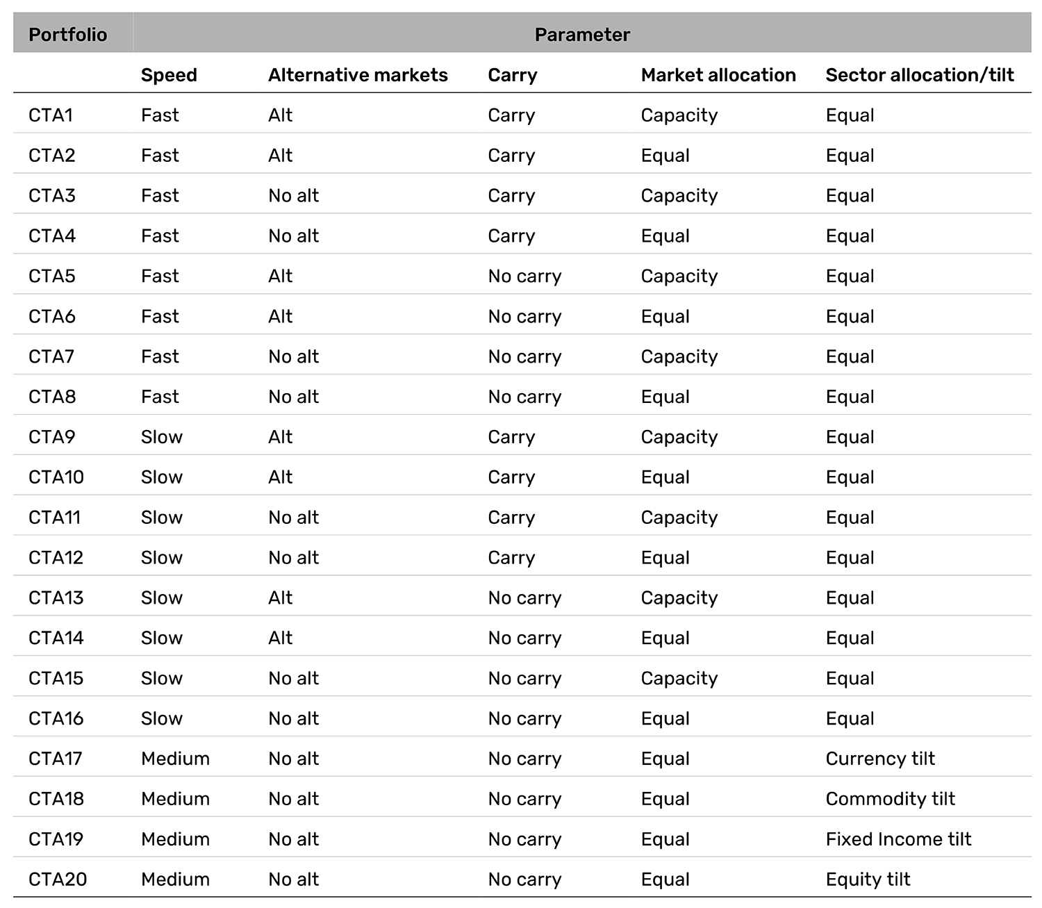
In a bid to model the dispersion we observe between index constituents, we have created a set of 20 trend-following proxies that we believe best capture the variations in the type of trend-following systems employed. We define a set of parameters, which our experience of trading these models for over 30 years suggests to us best represents the breadth of choices that trend followers typically contend with.

Below, we outline four binary choices to construct 16 (or 2⁴) core trend proxies:

1. Speed
   1. Fast: two-to-three month holding period, one-month lookback for position sizing
   2. Slow: six-month holding period, 12-month lookback for position sizing
2. Inclusion of carry
   1. No carry
   2. 15% allocation to currencies and fixed income carry
3. Inclusion of alternative markets
   1. Purely traditional: futures and FX forwards across commodities, currencies, fixed income and stocks (around 150 markets)
   2. Including alternative markets: such as power, synthetic credit indices and interest rate swaps
4. Allocations
   1. Equal risk weight: to each asset class (and equal risk weight to markets within each asset class)
   2. Proportional to capacity: based on daily dollar volume and exchange limits

In addition, we consider four additional trend-following proxies where we apply asset class tilts in the allocations step (4), bringing the total number to 20. In these proxies specifically, we ‘fix’ parameters one to three above to better isolate the impact of active allocation decisions. We do this by utilising a medium speed (four-month holding period), excluding carry, trading traditional markets only and applying equal market risk allocations within each asset class. However, instead of applying an equal 25% allocation to each asset class as we do in the first 16 proxies, we apply a 40% overweight to one of the asset classes and 20% to the remaining three.

The rationale for including these additional proxies stems from evidence that some managers consciously tilt their portfolios towards certain asset classes. In most cases, this active design choice is backed by the belief that particular asset classes or markets exhibit characteristics more conducive to a trend-following strategy, and an overweight would subsequently lead to a higher overall information ratio (IR). That being said, more nuanced cases also exist, where tilts are employed to solve for a specific use-case, such as optimising crisis performance.

The opposite school of thought to active tilts purports that all markets are equal in terms of their trend-following IR, and by that token, the goal should be to diversify risk across all markets. It is worth highlighting that the more sophisticated approach for proponents of this philosophy is to apply maximum diversification optimisation. This takes into account the covariance matrix of markets and, in the absence of constraints, skews allocations to less correlated markets. For the purposes of this paper, however, an equal-risk-weight approach (proxy parameter 4a, as outlined above) adequately proxies for this. In the presence of capacity constraints, however, predominantly arising from strategies with larger assets under management, the optimisation would tilt the weights towards higher capacity markets. Parameter 4b above is used to represent such cases.

Ironing out some final methodology points, we subtract an annualised transaction cost of 2% for fast and 1% for slow implementations, respectively, to account for turnover differences. We also apply a 1.5% management and 20% performance fee (with high watermark and end-of-year fee crystallisation, as is common) and assume 50% of cash is unencumbered, earning the Treasury bill rate.

Using this framework, in Figure 2, we replicate the analysis from Figure 1 but instead plot the annual performance for the 20 trend-following proxy portfolios. The bottom panel also similarly illustrates the difference between the best and worst annual performance for these trend proxies (aqua blue bars), alongside that of the actual SG Trend Index constituents (navy blue bars).

Figure 2: Proxy trend strategies, annual performance (2000-2024)⁵

Problems loading this infographic? - Please click here

Problems loading this infographic? - Please click here

Source: HFR, Inc., WithIntelligence, Bloomberg, Man Group Database. Date range: Jan 2000 – Dec 2024.

Overall, the results show that the proxy portfolios are reasonably robust in capturing both the yearly pattern of returns and dispersion, with the delta between the best and worst performers for each calendar year approximately in line with that of the actual SG Trend Index constituents. Further, if we adjust for those outlier SG Trend Index constituents whose approach deviated from the core trend-following principles, as referenced above, this alignment is even more pronounced. We can therefore leverage the insights from our proxy portfolios to better understand the practical dispersion between index constituents, as we will discuss in the following section.

Analysing the trend proxy portfolios and binary parameters

Taking a more holistic view of the long-term performance of each of our 20 proxy portfolios, in Figure 3, we observe that dispersion in the initial period from 2000 to 2006 is relatively less pronounced compared with the period following the onset of the GFC in early 2007. This is also visible in the annual performance dispersion between the proxy portfolios shown in Figure 2. The difference between the best and worst performers is below 10% in each of these years, with an absolute average pairwise correlation between the portfolios of 0.87. In sum, irrespective of the design parameters in the trend-following system over this period, trend followers largely enjoyed similarly positive returns. From 2007 onwards, however, this dispersion ticks up, as the equivalent correlation measure falls to 0.78.

Figure 3: Proxy trend strategies cumulative performance (2000-2024)

Problems loading this infographic? - Please click here

Source: Man Group Database. Date range: Jan 2000 – Dec 2024.

The more meaningful dispersion in the latter period stems from a combination of design choices. In the case of the market universe, the period following the GFC was widely regarded as the CTA winter, where traditional trend struggled amid the currents of the Federal Reserve put, while the proliferation of liquid, tradable alternative markets basked in plentiful trends. With regards to speed, the evidence is less clear, although we may posit that the whipsawing brought about by policy intervention was more conducive to a slower, passive approach. Carry and allocation differences also contribute to the uptick in dispersion, although the story boils down to more specific market environments in these cases. We will touch on this further shortly.

In any case, the primary takeaway from the long-term performance pattern is that different properties do well at different times. This analysis suggests there is no single ‘correct’ way to implement a trend-following portfolio and specific flavours may suit different investors’ preferences. For many investors, trend following’s role is seen as a diversifying, crisis-offset allocation, and therefore the parameters that drive outperformance in such periods play a crucial role in dispersion. To explore this, in Figure 4, we decompose the long-term performance between crisis and non-crisis periods to uncover which of the parameters give rise to improved crisis alpha properties.

We define crisis periods as the peak-to-trough time periods when the S&P 500 experiences a 15% or worse drawdown, in line with that of our earlier work. The y-axis corresponds to the full-period Sharpe, while the x-axis represents the crisis Sharpe. The diagonal line therefore signals where each proxy portfolio sits on this continuum.

Figure 4: Crisis versus non-crisis performance for the 20 trend proxies (2000-2024)

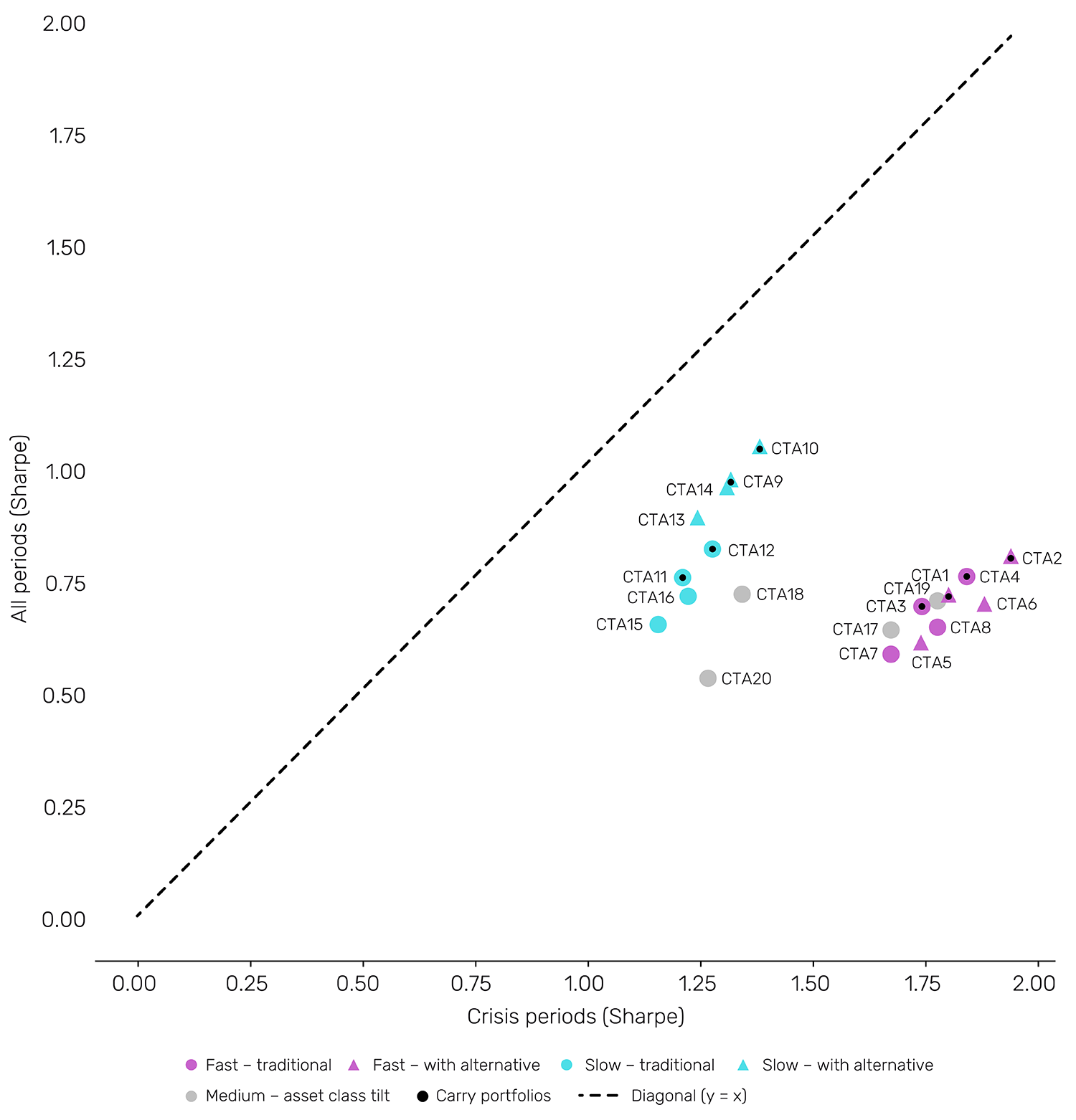
Source: Man Group Database. Date range: Jan 2000 – Dec 2024.

Our first observation is that all of the proxy portfolios sit below the diagonal line, underscoring that trend following’s crisis Sharpe is comparatively better than its non-crisis, and hence all periods, Sharpe. This accords with empirical evidence that trend following’s performance is most positive in the worst quintile of equity returns.

Where each of these portfolios sit below the diagonal line, however, is influenced by the different binary parameters of each proxy.

Speed

Starting with speed, a more well-documented binary parameter, and in keeping with the findings of our earlier paper The Need for Speed, we observe a clustering of faster trend (pink markers) further along the x-axis. This indicates that faster portfolios have historically tended to perform better during periods of crisis. This may also explain the higher dispersion between proxy portfolios that ticked up over 2007 and 2008 as the GFC equity sell-off escalated.

Alternative markets

Trading alternative markets, represented by the triangles in Figure 4, leads to better overall performance, as shown by the clustering of triangles in the top right-hand direction relative to the equivalent portfolios without alternative markets (circles). As discussed in a previous paper, alternative markets boast a wider range of more idiosyncratic price drivers, which leads to improved diversification throughout the full market cycle.

Notably, however, there is an interesting interplay with the effects of speed, with the additivity of alternative markets more apparent in slower trend systems. Kerson and Babbedge (2019) hypothesise that this could be because of the trading dynamics of alternative markets. This includes the larger presence of hedgers versus speculators, inelastic supply/demand and greater independence from risk on/risk-off or policy-based price action, which are conducive to more extended trends in alternative markets. A less reactive and turnover-heavy system may thus be better placed to capture these dynamics.

Asset class tilts

As discussed above, active asset class tilts can also drive meaningful bifurcation in trend-following outcomes and therefore serve as useful parameters to capture some of the variation that arises. In Figure 5, we plot the returns of the 20 trend-following proxies, highlighting in colour each of the portfolios that are tilted toward a specific asset class.

Notably, the relative performance between any of the asset class-tilted portfolios can be significant in any given year. 2019 is a pertinent example of this, when being overweight fixed income led to a marked improvement in performance relative to most other implementations. Despite this, there is no single asset class tilt that consistently outperforms year-after-year, although patterns do emerge in a handful of years, as evidenced by the tilted portfolios appearing at the edge of the distribution in similar market environments.

Returning to Figure 4, portfolio CTA17 (currency tilt) and CTA19 (fixed income tilt) sit among the cluster of fast (pink) portfolios that outperform in crises, despite deploying a ‘medium’ speed. This corroborates the outperformance of the royal blue (currencies) and maroon (fixed income) dots from Figure 5 in years marked by crises, including 2002, 2008 and 2022, where generally long US dollar and long fixed income positions outperformed (during the dot-com bubble burst and GFC). Conversely, short fixed income was particularly additive during the recent inflationary episode.

Figure 5: Proxy trend strategies’ annual performance, focusing on asset class tilts

Problems loading this infographic? - Please click here

Source: Man Group Database. Date range: Jan 2000 – Dec 2024.

Carry

Those less accustomed to trend following may question why carry is in the scope of this analysis. It is not a traditional trend-following signal after all. Trend followers, at least in our investigation of the group of SG Trend Index constituents, often complement their core trend allocation with a satellite allocation to diversifying, non-trend content. In doing so, they aim to provide diversifying performance during more challenging periods for trend signals. Carry is a natural fit to achieve this, given that stable, rangebound markets, which are not conducive to most trend signals, are often associated with beneficial periods for carry. Interestingly, however, slower trend signals do resemble the properties of carry.

The size of allocation to non-trend content, and therefore carry, is also variable among trend followers, and is largely dependent on the profile of returns an investor is seeking to achieve. While we make no claims as to how much is ‘best’, from a dispersion point of view, the allocations have a meaningful impact on performance in some years, as shown by the clustering of purple points at the extremes of the distribution in Figure 6. In 2016 and 2023, for example, an allocation to carry was beneficial. Specifically in 2023, carry was a key reason for some proxies finishing in positive territory, with higher-for-longer rates in the US leading to profitable FX and fixed income carry positions versus countries maintaining or moving towards lower rates, such as Japan. As it pertains to crisis performance, however, the split of grey markers in Figure 4 between both the pink (fast) and aqua blue (slow) clusters indicates that carry does not have a material impact, with other parameters being a more prominent driver of crisis period dispersion, as described above.

Figure 6: Proxy trend strategies’ annual performance, including and excluding carry

Problems loading this infographic? - Please click here

Source: Man Group Database. Date range: Jan 2000 – Dec 2024.

Conclusion: Subtle differences, significant outcomes

Our analysis in this paper illustrates that even among seemingly similar trend-following CTAs, subtle differences in key parameters – such as speed, market set, carry and allocation methods – can drive considerable performance dispersion, particularly during periods of heightened market stress. The different combinations of these binary parameters, implemented through the 20 proxy portfolios, do a robust job in capturing the actual range of returns from constituents of the SG Trend Index. In that sense, we would argue that they offer a behind-the-scenes insight into the mechanics of the SG Trend Index universe, while also serving as a novel framework for internal benchmarking and supporting continued refinement in risk management.

Appendix

1. Constituent data is sourced from third-party databases with which Man Group has a data licence.
2. Trend-following strategies involve substantial risk of loss, including the potential loss of principal. These complex strategies utilise derivatives and alternative markets and may not be suitable for all investors. Leverage can significantly amplify losses. Past performance does not guarantee future results.
3. See: https://wholesale.banking.societegenerale.com/fileadmin/indices_feeds/ SG_Trend_Index_Constituents.pdf
4. See: Harvey, C.R., E. Hoyle, S. Rattray, M. Sargaison, D. Taylor, and O. Van Hemert (2019) “The Best of Strategies for the Worst of Times: Can Portfolios be Crisis Proofed?”, Journal of Portfolio Management, 45(5), 7-28. And for the most recent selloffs see: Harvey, C.R., E. Hoyle, S. Rattray, and O. Van Hemert (2020) “Strategic Risk Management: Out-of-Sample Evidence from the COVID-19 Equity Selloff”, working paper.
5. A CTA is a type of hedge fund that uses a managed futures strategy, primarily investing in futures and options contracts across various markets such as commodities, currencies, interest rates and equity indices.