Limitations of Liquidity Risk Frameworks

1. Introduction

Portfolio liquidity, and the way in which the fund industry considered it, has been changed forever by the events of the past few years. Since 2018, a few large funds suspended all subscriptions and redemptions after they experienced a high level of redemption requests. While these events highlighted the importance of measuring and monitoring liquidity risk as a fundamental part of risk management, there is still no consensus on which approach, of the many that exist, is optimal.

So, we decided to investigate some best practices around liquidity risk, with a focus on two key areas:

• The risk management toolkit needed to monitor, analyse and control liquidity risk;
• The limitations of these tools and how investors can address these limitations.

2. Risk Manager Toolkit to Monitor Liquidity Risk

At a fund management level, liquidity risk is defined as the risk that a fund cannot return investors’ money within a time period determined by the fund’s mandate or by regulation.

For clarification, liquidity risk is not related to how much money the fund would lose should market liquidity conditions dry up, as observed such in March 2020. The aim here is to focus solely on the ability of funds to perform their obligation to give investors’ money back on time, should redemptions occur in an environment of reduced liquidity.

2.1. Liquidity Profile

An efficient approach to quantify liquidity risk is to estimate how many days it may reasonably take to liquidate a position under normal market conditions, without materially impacting market prices. If we could calculate a measure of liquidity for all positions in the portfolio, we could determine a measure of portfolio liquidity – commonly known as a liquidity profile.

For transparent markets, where information is readily available, this calculation is relatively straightforward. In these instances, one parameter which is often considered is the participation rate, which represents how much of the average daily volume (‘ADV’) one could reasonably expect to trade in one day without significantly moving the market prices. A typical participation rate is less than 10%. It is also good practice to assess the actual average participation rate of a specific fund to get an idea of where the fund manager market activity stands versus the available liquidity.

For less transparent markets, such as corporate and high yield bonds, less information is generally available. Here, some creative quantitative methods are often necessary to quantify the liquidity profile. For example, these methods can leverage the use of large data sets such as bond bid-offer runs.

2.2. Balanced Versus Unbalanced Profiles

When liquidating a portfolio, a critical decision that needs to be made concerns the risk profile the fund will target upon liquidation. It is important to distinguish between an unconstrained or unbalanced execution from a constrained or balanced execution.

An unconstrained execution means that the fund exits a position based on the available market liquidity. As an example, let’s assume a participation rate of 10%. In this scenario, the fund liquidates whatever it can, when it can, using the participation rate assumption. In the unbalanced example, the fund will sell any long-position security when there is a buyer for it at the assumed participation rate.

On the other hand, a constrained execution means that the fund exits positions under the constraint of having to maintain a similar overall liquidity risk profile in the portfolio after execution.

To illustrate, assume a hypothetical portfolio holds two assets, A and B, in equal weight. We also assume an extreme case where A is liquid whilst B is very illiquid. The unbalanced approach assumes the portfolio manager sells asset A in a single day, because it can, whilst the balanced approach forces the portfolio manager to sell both assets A and B at the same time in order to maintain a proportionate allocation.

The balanced approach, which assumes that the liquidity risk is relatively constant during the whole liquidation process, will take longer because liquidating B in one day might be a challenge. We understand that this example is not practical, since practitioners would most often liquidate a fund in an unconstrained and unbalanced way as opposed to a constrained and balanced way due to the fund management company’s obligation to return the funds to investors as soon as possible. However, this example highlights the difference between a balanced and unbalanced liquidation.

2.3. Liquidity Stress Testing Framework

Stressing liquidity profiles is an important exercise which needs to be performed on a regular basis. Liquidity stress testing (‘LST’) provides confidence that the fund can fulfil its obligations towards its investors even under the worst assumptions. LST means taking extreme, painful and violent scenarios both in terms of liquidity shocks and redemptions. To that effect, we usually distinguish between two types of stress methodologies. The first type of LST is based on assumptions and those need to be severe enough for the LST to be useful. The second type of LST is based on historical scenarios. For the LST to be complete, it is important to perform both types of stresses.

In addition, it is also important to distinguish two types of stresses when it comes to LST: assets and liabilities.

2.3.1. Asset-Side Stress Tests: Liquidity Shock Scenarios

Asset-side stress tests shocks the actual liquidity of the assets. These scenarios aim to shock the available liquidity by either updating (often reducing) the participation rate or assuming liquidity conditions which are more adverse. This kind of environment can often be observed around year end, when liquidity is more muted. Below, we set out some examples to illustrate which types of such scenarios can be implemented, based on assumptions or based on historical data:

• Assumption based: update the participation rate from 10% ADV to 5% ADV;
• Historical based: update the ADV from using current market conditions to another period which can be less liquid, such as year-end.

2.3.2. Liability-Side Stress Tests: Investor Redemptions

Stressing liabilities is about stressing the redemptions we could see in a fund. Those types of scenarios shock the funds under management. Below, we provide some such scenarios which can be implemented, based on assumptions or on historical data.

• Assumption based: 50% institutional investor and 35% retail/pensions redemption in one day;
• Assumption based: top three investor redemptions in one day;
• Historical based: maximum 1-day historical redemption since inception in one day;
• Historical based: maximum 1-month redemption since inception in one day.

The details in these examples are adjustable – the point is that having a large set of diverse stress scenarios is a key internal liquidity risk control.

3. Limitations of the Risk Manager Toolkit and How to Address Them

3.1. Checking Volumes Input Data Make Sense

Some funds are more difficult to model from a liquidity standpoint. For example, eventdriven and risk arbitrage positions are less straightforward because it is standard to see volume drying up upon a deal announcement.

But does the data back this belief that liquidity traded volume is reduced for several arbitrary securities related to mergers and acquisitions? Figure 1 focuses on a hypothetical portfolio made of arbitrarily chosen and equally weighted of announced M&A deals. It quantifies how the ADV of this basket evolves as a function of time, measured in days. Every security in that portfolio is displayed in its own time space where time t=0 represents the announcement date of the M&A deal. In addition, the ADV is normalized to 1 at date -150 day. Finally, the data is split into three buckets: the large, medium and small caps using 33 and 66 percentiles.

Figure 1. Percentage Average Daily Volume for M&A Target Companies (465 Stocks)

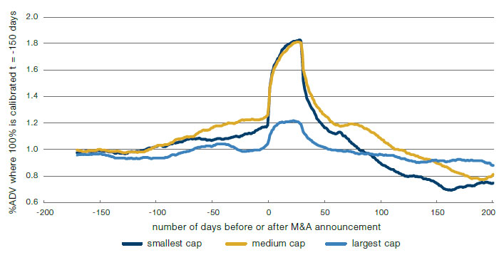
Source: Man Group; as of 30 July 2020.

As expected, the chart shows an explosion in volumes just after announcement. After reaching a peak in ADV, there is a reduction in traded volumes. However, this does not necessarily mean that the liquidity profile is materially worsening. For example, there would often still be a buyer of the stocks for announced deals if the seller is willing to accept a discount to the M&A spread which is trading, an effect not easily captured.

3.2. Challenging the Liquidity Model Assumptions

Different liquidity models are sensitive to modelling assumptions and these sensitivities need to be well understood. A good way to check the model validity of results and know where to dig further in order to improve the model is to compare different model outputs. Figure 2 shows a comparison of results between different liquidity models for three hypothetical portfolios (Fund 1, Fund 2, Fund 3), which are comprised of assets for which we believe the liquidity is the most challenging to assess. Each point represents a security and displays how long it would take to liquidate it, in days. In abscissa, we use ‘model 1’, which is sensitive to the market impact parameter – a measure of how much one might move the market upon trading. In ordinates, we use ‘model 2’, which is predominantly sensitive to ADV. If the two models are in line, the plot will be close to the 45-degree angle line below.

Figure 2. Liquidation Model Comparison

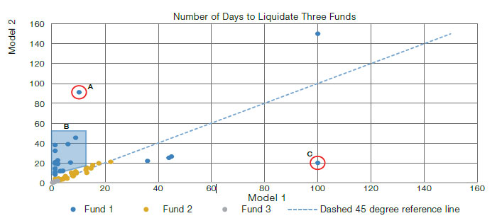
Source: Man Group. For illustrative purposes only.

For Fund 1 (a bond fund), for which liquidity is difficult to compute, model 2 is generally more conservative than model 1. Model 1 predicts that sizeable positions can be sold in a couple of days, in some cases 14% of an issue (point A). When looking into the results, model 1 looks to be very dependent on the market impact parameter. The data is based on a 2% price impact (which is slightly above the weighted average bid offer at the time of running). Model 1 suggests that out of all the bonds in a USD1- billion hypothetical portfolio, only a few bonds would take over a day to liquidate, which seems unlikely (highlighted in light blue area B). In addition, we believe model 2 captures better the liquidity of the anomalous position (point C). This is because the results are in line with the quantity of dealers that are providing 2-way quotes of reasonable size for that security.

The two models’ coverage of Funds 2 and 3 exhibit a closer relationship with a tolerable level of difference.

3.3. Challenging the Stress Assumptions

LST uses a diverse set of scenarios. Some of those scenarios are historical and some of those scenarios are based on assumptions. Whenever an assumption is used in a stress scenario, it is important to check that it makes sense, so the scenario is properly calibrated.

For example, one may use scenarios with an x% institutional investor redemption and β * x% retail investor redemption. We believe fund managers should estimate a proper β to use in a liquidity stress scenario. It is generally accepted and observed by practitioners that retail investors are more latent and captive than institutional clients, so the practitioners would expect β <1. Does the data verify that belief?

Figure 3 shows the results of a regression analysis of historical redemptions using a Least Square Method:

redemption_retail_t = β * redemption_institutional_t + ϵ

where t represents the month ‘t’.

Figure 3 shows the scatter plot, where the x-axis represents a measure of monthly institutional redemptions and the y-axis represents a measure of monthly retail redemptions. Note that the redemptions have been normalised. We combined 60 months of data across five business units (so 300 points in total) as well as the best fit regression line (dotted line), which confirms the belief that retail investors are more latent than institutional investors and the β estimation is less than 1. In addition, this result is statistically significant.

Figure 3. Regression of Monthly Institutional Redemptions on Monthly Retail Redemption Flows

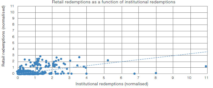
Source: Man Group; as of 31 December 2019.

3.4. Comparing Fund Liquidity Against Competitors

13F disclosures of similar funds and competitors can be used to assess liquidity progress of a specific fund versus its competitors. Again, we believe this is an important piece of information which can give some comfort around what kind of profile is acceptable. Figure 4 shows such an example performed for a fund against competitors using this method.

Figure 4. Liquidity Profile of Competitors

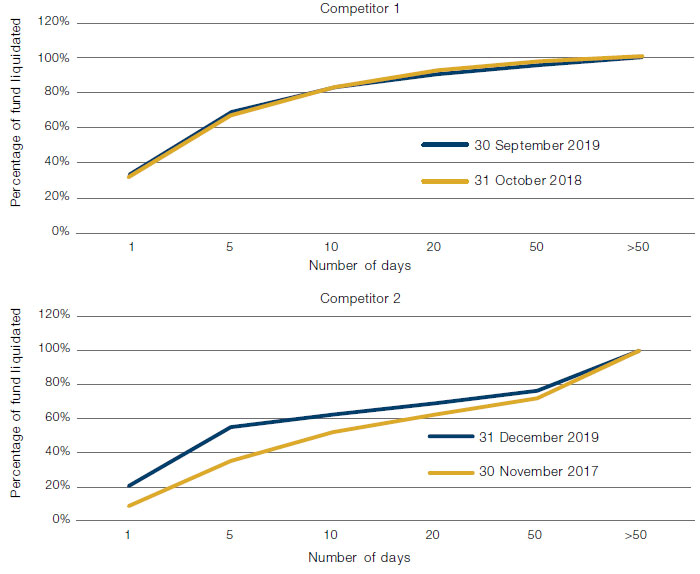
Source: Man Group; as of 31 July 2019.

4. Conclusion

Establishing a methodology for measuring the liquidity profile of funds, and stresstesting these profiles, is fundamental to controlling liquidity risk. In our opinion, an effective risk management framework should also formally challenge the results – comparing them with the views of key stakeholders and find other sources of information. It is important to note that a one-size-fits-all approach is likely to be littered with errors given the diverse range of funds that exist. Developing a tailored approach, such as those outlined in this report, is essential for capturing the nuances of each fund’s liquidity risk exposure and model limitations.