Introduction: Options Are Not Your Only Option
Managing portfolios in times of crisis used to be simple. Or so the thinking went. When market returns looked like they would fall, you would buy bonds and let the uncorrelated diversification take care of the rest. But in an environment where bonds and equities have fallen in tandem, investors have had to shift their reliance on fixed income – which was nonetheless very expensive – to other assets and strategies.
Our research shows that systematic strategies can offer a meaningful alternative to negative carry options.
The first ports of call are often tail hedges by way of similarly expensive equity put options. If we think of tail hedging as a way of outsourcing portfolio risk management to market makers, when the costs become as high as they have been in the recent selloffs, bringing risk management back in house should be a serious consideration. Our research shows that systematic strategies including trend-following, quality factors, or direct portfolio overlays can offer a meaningful alternative to negative carry options.
We’ll admit, the usefulness of systematic strategies in times of crisis is not a new finding. In a Man Group academic paper The Best Strategies for the Worst Crises, trend-following and equity factor portfolios based on signals such as profitability, leverage and growth both showed strong defensiveness traits. These strategies show positive returns in crises, but unlike tail hedging attempts, have not suffered from poor returns outside of equity market drawdowns. Other ‘crisis strategies’ might also include risk-mitigating futures overlays that use risk controls such as volatility scaling, momentum and cross asset correlations.
The key difference to highlight here is that systematic strategies may or may not be defensively positioned at any given moment. Tail hedges on the other hand are always short the market and so are dependent on a certain outcome. This leaves investors with a problem. Do you choose an always on, negative carry tail hedge strategy or do you choose systematic-based strategies which generate exposures over time? The answer lies in portfolio ‘convexity’ – a measure investors can use to determine just how responsive different strategies are to market crises.
What is Portfolio Convexity?
While the term convexity is frequently used in describing options-based strategies, it’s not always clear what this means in practice. A straddle (buying a put and call of the same strike and maturity) yields an option strategy with convexity in market up or down conditions. The payoff profile looks like the bold green line if we assume no cost (Figure 1). However, straddles are not costless. The dotted line represents the payoff less the premium loss. While the chart appears favourable in markets with low to average volatility, those losses add up over time. Many argue the volatility premium is a form of positive carry strategy that exists from hedgers overpaying for options.
Figure 1. The Return Profile of an Options Straddle Adjusted for Costs
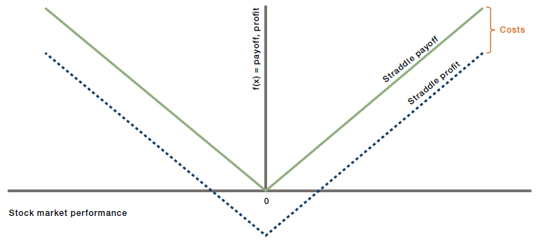
For illustrative purposes only.
The expected payoff above is for any one trade, an oversimplification in a world of multi-asset, multi-strategy portfolios. Over time, premia for a straddle and equity returns vary. Figure 2 shows historical returns for rolling one-month straddles plotted against 1-month returns for the S&P500 Index. A second order polynomial trend line provides a view of the convexity profile of this long straddle programme.
Figure 2. Monthly Returns: Rolling 1-Month ATM Straddle on S&P 500
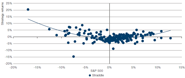
Source: Bloomberg data, Man Group calculations. Monthly data, May 2007 to September 2022. Please see the important information linked at the end of this document for additional information on hypothetical results.
Actual trading never follows theory perfectly. However, there seems to be strong convexity on the left tail, with a more moderate amount on the right tail; a not unsurprising result as markets tend to fall quickly and rise more slowly. As such, the long straddle shows consistently less return in rising markets, but much larger and more frequently positive returns in a decline. Unfortunately, this strategy comes with a cost: a mean monthly return of -17 basis points. Buying options delivers the portfolio convexity you might be looking for, but at a clear cost to overall performance.
Buying options delivers the portfolio convexity you might be looking for, but at a clear cost to overall performance.
Enter systematic strategies such as trend-following. Drawing once more on the findings of The Best Strategies for the Worst Crises, we can see how trend-following strategies performed during different quintiles of equity returns. Trend strategies have shown the historically strongest annualised returns in the worst and best quintiles respectively (Figure 3). Once again, we can see the ideal ‘convexity smile’ of a strategy that is expected to perform best at extreme ends of market performance, with a preference for protection on the downside.
Figure 3. Simulated Returns of a Trend-Following Strategy from Worst to Best Equity Environments
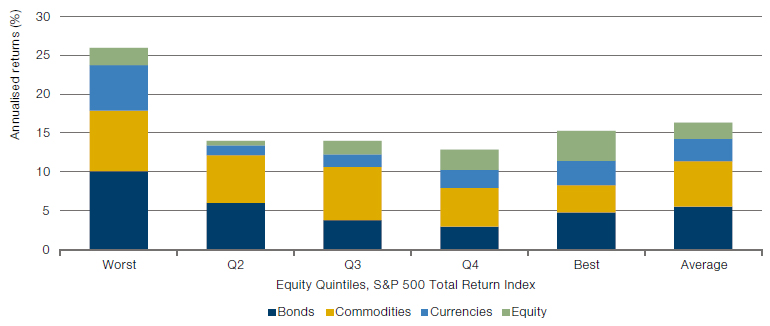
Source: Man Group calculations. For illustrative purposes only. The figure shows the annualised average trend return for rolling 3-month windows, attributed to the four asset classes covered, under different general equity market conditions. The results are reported for equity market quintiles, with quintile 1 corresponding to the worst 3-month S&P 500 returns and quintile 5 to the best. The right-most bar corresponds to the average return across all periods. Returns do not include interest income, i.e. can be considered excess returns, and are gross of transaction costs and fees. Research derived from Man AHL paper, Trend Following: Equity and Bond Crisis Alpha, where Man AHL studies trend-following strategies in bonds, commodities, currencies and equity indices between 1960 and 2015. The simulated performance data above reflecting hypothetical results is shown for the time period from January 1, 1960 to December 31, 2015. Please see the important information linked at the end of this document for additional information on hypothetical results.
While for years adding bonds has been the “correct” corrective mechanism for portfolios, more recent inflationary periods have been different.
One important feature of trend is that it generates those returns across asset classes. While an equity options strategy seeks returns solely from moves in that specific equity market, trend positions are diverse. In times of market recovery following a sharp correction, not all asset class returns revert as sharply as equities often do. Therefore, a multi-asset exposure strategy such as trend-following helps retain profits as markets recover for two reasons; it either improves upon an investor’s portfolio by diversifying it or it reduces risk in asset classes the investor owns.
While for years adding bonds has been the “correct” corrective mechanism for portfolios, more recent inflationary periods have been different. Meaningful downtrends in bonds have led to momentum strategies shorting bonds which behaves like a corrective measure to traditional bond/equity portfolios. This dynamic use of bonds is helpful for traditional 60/40 investors who might only rarely short bonds. Meanwhile, long exposure in commodities in 2022 has provided some level of portfolio protection from inflation.
Options Versus Trend
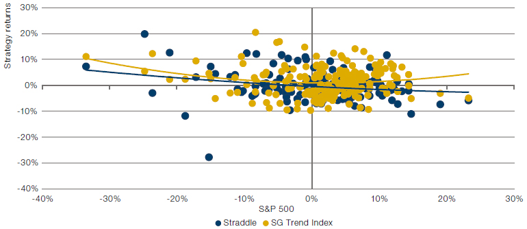
So how do trend returns compare to options straddles? Interestingly, on a one-month basis a straddle strategy shows more convexity, albeit still at a negative cost to average returns (Figure 4). However, on a three-month rolling basis we see the convexity winners reversed (Figure 5). Trend-following delivers better returns in both extreme down and up markets for the S&P 500 while still delivering a positive average return overall (0.51%). Trend avoids the option premium in the right-hand tail and the high cost of an investor having to roll into new options straddles each month.
Figure 4. Monthly Returns: S&P 500 Straddles vs. SG Trend Index
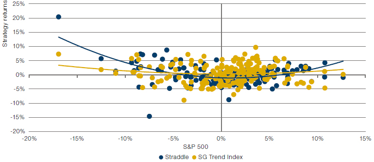
Source: Bloomberg data, Man Group calculations. Monthly data, May 2007 to September 2022. Please see the important information linked at the end of this document for additional information on hypothetical results.
Figure 5. Rolling 3-Monthly Returns: S&P 500 Straddles Vs. SG Trend Index
Source: Bloomberg data, Man Group calculations. Monthly data, May 2007 to September 2022. Please see the important information linked at the end of this document for additional information on hypothetical results.
Creating Downside Convexity Profiles
We might look to strategies that generate downside convexity and skip upside returns.
While trend-following strategies display convexity in both up and down equity markets, most investors thinking about convexity tend to consider it in the context of risk-mitigating strategies. Thus, while trend-following upside returns help the strategy generate returns in both up and down markets, it tends to do so through being long risk assets like equities and commodities alongside being long riskier currencies. As such, we might look to strategies that generate downside convexity and skip upside returns.
In Figure 6, we can see the returns profile of a rolling one-month S&P 500 95% put strategy against monthly S&P 500 returns. The trend resembles the well-known ‘hockey stick’ from options theory textbooks, with higher strategy returns heavily skewed towards extremely negative market performance i.e. the left tail. Similar to the findings in our previous paper, the overall average monthly return of this strategy is negative (-0.18%) therefore running rolling 95% puts quickly becomes expensive.
Figure 6. Monthly Returns: Rolling Monthly 95% Puts Vs. S&P 500
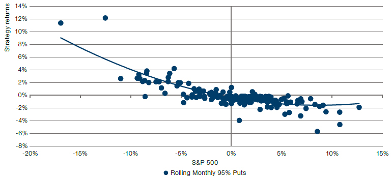
Source: Bloomberg data, Man Group calculations. Monthly data, May 2007 to September 2022. Please see the important information linked at the end of this document for additional information on hypothetical results.
The Best Strategies for the Worst Crises compares a whole host of defensive strategies ranging from buying puts and credit default swaps, to gold and beyond. Over time, the hedging strategies tend to show negative returns (Figure 7) with the more directly short an asset is positioned – such as puts or CDS – the worse the long-term performance. This difference in performance is relatively intuitive as over time risk premia are earned from long exposure to equities, bonds, and credit.
Figure 7. Cumulative Total Return of Selected Defensive Strategies
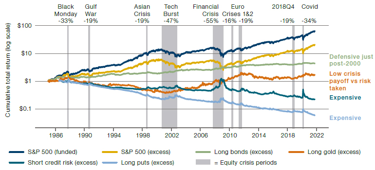
Source: Bloomberg data, Man Group calculations. The periods selected are exceptional and the results do not reflect typical performance. The start and end dates of such events are subjective and different sources may suggest different date ranges, leading to different performance figures.
Using long puts as our starting point, we can compare the relative strength of alternative defensive strategies such as trend-following and the equity quality factor. In equity market drawdowns, stocks that exhibit stronger profitability and growth characteristics have consistently delivered positive returns in these crisis periods. Figure 8 shows the total and annualised return of Profitability (beta-neutral) stocks across different market drawdown periods relative to long puts, short credit risks and different trend-following strategies.
Figure 8. Trend, Quality and Options Performance in Crisis Periods
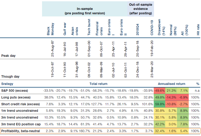
Source: Bloomberg data, Man Group calculations. Data from 1985 to 30 September 2021. The periods selected are exceptional and the results do not reflect typical performance. The start and end dates of such events are subjective and different sources may suggest different date ranges, leading to different performance figures.
QMJ shows very little convexity, performing more like a short beta strategy.
In analysing convexity, we use the Quality Minus Junk (‘QMJ’) factor as our benchmark quality factor to compare its returns with equity puts and the S&P 500 (Figure 9). Intriguingly, while returns in down months are similar, QMJ shows very little convexity, performing more like a short beta strategy. However, unlike options, the factor generates 0.53% monthly returns versus the -0.18% return of short puts. Importantly for hedgers, the strategy acts as a “first responder” by generating returns often as quickly as options strategies.
Figure 9. Monthly Returns: Rolling 95% Puts Vs. Defensive Equity
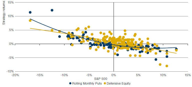
Source: Bloomberg data, Man Group calculations. Monthly data, May 2007 to September 2022. Please see the important information linked at the end of this document for additional information on hypothetical results.
Applying Systematic Overlays
Having looked at portfolio diversifiers like trend and quality, we now turn our attention to more direct risk mitigation tools that introduce controls into a long only asset portfolio to generate convexity. In the book Strategic Risk Management, volatility scaling is analysed as a potential risk controlling overlay. A volatility-based risk overlay seeks to reduce exposure to underlying assets as the volatility of those asset classes or portfolios increases. When observing daily equity returns over the past century, the authors identified that volatility increases are not only persistent but also tend to be more clustered than isolated (Figure 10).
Figure 10. Volatility Clusters: Daily US Equity Excess Returns
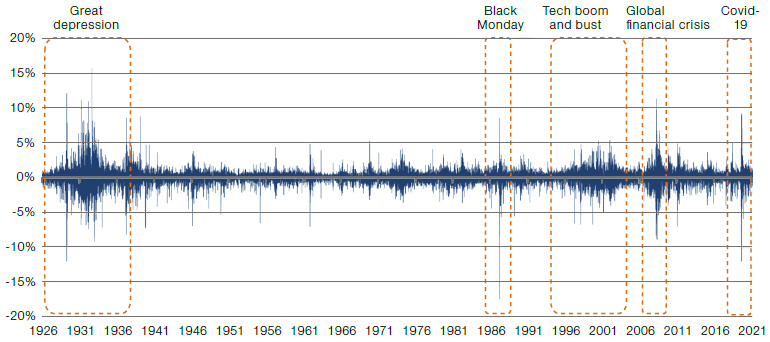
Source: Man AHL, Kenneth R. French data library. Equity represented by value-weighted returns of firms listed on NYSE, AMEX and NASDAQ. The periods selected are exceptional and the results do not reflect typical performance. The start and end dates of such events are subjective and different sources may suggest different date ranges, leading to different performance figures.
Applying volatility scaling, alongside other risk-reducing portfolio overlays, can help investors adapt their gross long exposure according to different systematic triggers. However, while these hypothetical exposures appear dynamic over time, they do little to tell us if the introduced risk controls add convexity or return to the portfolio. To do this, we can use the baseline static strategic asset allocation of the above portfolio and then subtract the returns of the static portfolio from the dynamic one. The difference in returns will be entirely a result of the dynamic overlays. Plotting those returns alongside the same equity put programme versus S&P 500 returns yields interesting results on a 1- and 3-month basis (Figures 11 and 12 respectively).
Figure 11. Monthly Returns: Monthly Puts Vs. Overlays
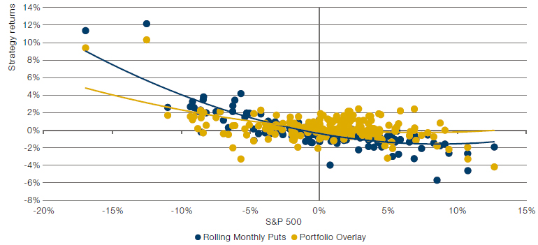
Source: Bloomberg data, Man Group calculations. Monthly data, May 2007 to September 2022. Please see the important information linked at the end of this document for additional information on hypothetical results.
Figure 12. Rolling 3-Monthly Returns: Monthly Puts Vs. Overlays
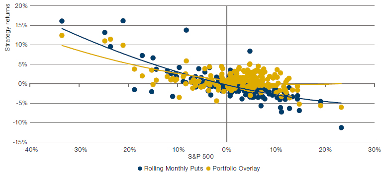
Source: Bloomberg data, Man Group calculations. Monthly data, May 2007 to September 2022. Please see the important information linked at the end of this document for additional information on hypothetical results.
Convexity for the overlays comes from their ability to add risk.
These returns show positive convexity for both strategies with very similar left tail characteristics for both; however, markedly improved right tail characteristics for portfolio overlays versus puts. Overlays also come out on top with a positive 0.44% mean monthly return against -0.18% for puts. The mild right tail convexity for the overlays comes from their ability to add risk at times to the portfolio and thus benefit from the risk premia of the underlying asset classes. The results should not be too surprising as risk controls based on volatility scaling effectively replicate volatility and market exposures of options. Volatility is after all the input for both options and volatility scaling.
Combining and Creating Portfolios of Risk Mitigating Strategies
The above strategies generate exposures and returns in different ways. While each has shown efficacy over time in generating positive returns in crises, investors may be reluctant to rely on any one strategy to ensure the robustness of their risk mitigation programmes. A combination of approaches may provide more certain outcomes and thus more confidence in the success of the programme. As a rough measure, we combine the three approaches: trend, QMJ and portfolio overlays into an overall programme with a simple 33.3% allocation of exposure to each. Once again, options deliver better convexity on a one-month basis, but systematic strategies almost fully catch up on a 3-month basis while providing a better average monthly performance.
Figure 13. Monthly Returns: Monthly Puts Vs. Combined Systematic Approach

Source: Bloomberg data, Man Group calculations. Monthly data, May 2007 to September 2022. Please see the important information linked at the end of this document for additional information on hypothetical results.
Figure 14. Rolling 3-Monthly Returns: Monthly Puts Vs. Combined Systematic Approach
Source: Bloomberg data, Man Group calculations. Monthly data, May 2007 to September 2022. Please see the important information linked at the end of this document for additional information on hypothetical results.
Combining Systematic and Options Hedges
While results look acceptable over longer time horizons, a challenge for risk mitigation portfolio managers is ensuring crisis returns in short-term market shocks without generating the long-term negative carry of an options programme.
A challenge for risk mitigation portfolio managers is ensuring crisis returns in short-term market shocks.
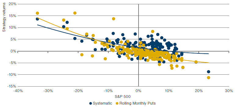
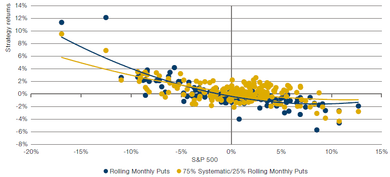
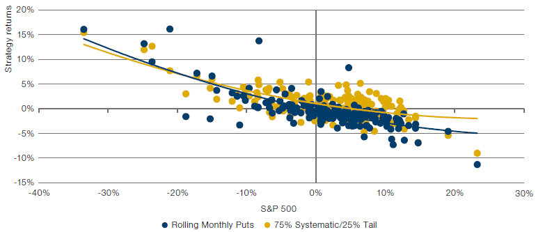
Given the positive returns of systematic strategies over time, a portion of those returns/alpha could be invested into a partial options-based hedge programme to enhance the responsiveness of the risk-mitigating portfolio. Many levers can be used to allocate to options; however, a simple starting point of 25% to tail hedging yields a slight reduction in overall average monthly returns from 0.42% to 0.32%, the convexity profile nearly wholly overlaps that of the rolling puts (Figures 15 and 16). At a stroke, investors can replicate the downside convexity profile of put options but without the carry.
Figure 15. Monthly Returns: Monthly Puts Vs. Systematic & Tail Hedges
Source: Bloomberg data, Man Group calculations. Monthly data, May 2007 to September 2022. Please see the important information linked at the end of this document for additional information on hypothetical results.
Figure 16. Rolling 3-Monthly Returns: Monthly Puts Vs. Systematic & Tail Hedges
Source: Bloomberg data, Man Group calculations. Monthly data, May 2007 to September 2022. Please see the important information linked at the end of this document for additional information on hypothetical results.
Conclusion
The multi-asset nature of trend-following helps provide much-needed diversification to a tail hedging strategy.
Creating genuine convexity is no simple task. When looking for a strategy to perform best at the extreme ends of market returns, investors often turn to guaranteed but expensive put and call options to provide convex returns. The multi-asset nature of trend-following helps provide much-needed diversification to a tail hedging strategy – not least in an environment where traditional diversifiers such as bonds have become increasingly correlated to mainstream equities.
Building on our previous research into the optimal strategies for market crises, including trend-following and the equity quality factor, we have found that sophisticated systematic overlays, combined with a small allocation to tail hedge options, can deliver an almost identical convexity profile at an improved rate of average monthly returns.
For investors concerned about future sudden market selloffs, preparation is key. Options are only part of the solution, not the whole, and building resilient risk-mitigation strategies takes time and care. Market selloffs are often far sharper than sudden market gains and so downside convexity strategies need to be stress tested for the worst crises.
You are now leaving Man Group’s website
You are leaving Man Group’s website and entering a third-party website that is not controlled, maintained, or monitored by Man Group. Man Group is not responsible for the content or availability of the third-party website. By leaving Man Group’s website, you will be subject to the third-party website’s terms, policies and/or notices, including those related to privacy and security, as applicable.