Introduction
Ubiquitous: adj., meaning present, appearing, or found everywhere.
Examples surround us, such as cars or computers or smartphones. Glasgow’s ‘The Ubiquitous Chip’ eatery is now so well-known it is simply referred to by locals as ‘The Chip’. In asset management, there are few terms more ubiquitous than the 60/40 portfolio. Indeed, like ‘The Chip’, the superfluous ‘portfolio’ is dropped and it is now just referred to as ‘60/40’.
Ubiquitous items are often taken for granted. There have been numerous articles criticising 60/40 in the media recently, so we thought it appropriate to do a little investigation. In this article, we consider the history of 60/40 and how the strategy can be adapted to respond to a world where both of its performance drivers – bonds and equities – appear expensive relative to the past. We pay particular attention to fixed income by analysing markets back to 1960 in order to incorporate a period of rising rates; an outcome which many investors believe is likely to materialise looking forward, and which is often missed in studies only spanning the past few decades. We believe investors need to embrace active management via risk rather than notional investing, and market-timing overlays such as trend-following.
What Is 60/40?
The term 60/40 refers to a portfolio which has 60% invested in equities and 40% in bonds. This is in capital terms, with no leverage. In theory, at least, it is supposed to be more balanced than a pure equities investment. This is because in times of equity market stress, a flight to the safety of bonds is supposed to cushion the equity losses. It appears not to be just a theoretical construct either; at Man Group, it is our experience that 60/40 is often a good proxy for many investor portfolios.
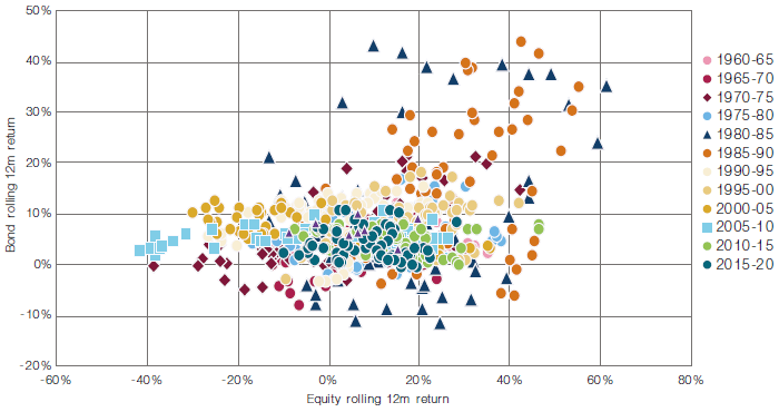
Figure 1 illustrates what makes equities and bonds the Bert and Ernie of the asset management world. We have chosen MSCI World Equities to represent equities and Bloomberg Barclays Global Aggregate for bonds. Before inception of these indices, we use the equity and fixed income data from Hamill et. al. (2016) in order to include the period during the 1970s and 1980s when fixed income total returns were negative. Note how:
- The bulk of returns are in the (profitable) top-right quadrant;
- When equities or bonds are negative, the other tends to be positive (see equities in the 2005-10 cohort, or bonds in the 1980-85 cohort);
- There are relatively few cases of bonds and equities being simultaneously negative (bottom-left quadrant).
Figure 1. Rolling 12-Month Equity and Bond Trailing Returns by 5-Year Cohort
Source: Man Group database, Bloomberg, MSCI. Date range: 1 January 1960 to 31 August 2020.
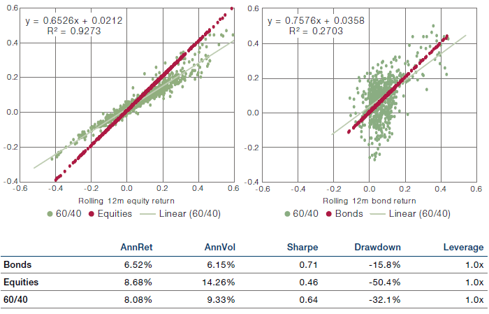
Once we take the 60/40 weightings into account, however, a few cracks appear. Figure 2 illustrates the 60/40 rolling 12-month return as a function of both equities (LHS) and bonds (RHS). 60/40 is 93% correlated to equities alone, and only weakly correlated to bond returns. The reader that looks at Figure 1 and sees the logic of investing in portfolios of equities and bonds, is not implementing this strategy with a 60/40 portfolio, in our view. The reason for this, of course, is that not only do we have 50% higher notional allocation to equities over bonds, but equities are much more volatile than bonds – 14% versus 6%, according to our dataset.
Figure 2. Rolling 12-Month 60/40 Returns (Green) Versus Equity Return (LHS) and Bond Return (RHS)
Source: Man Group database, Bloomberg, MSCI. Date range: 1 January 1960 to 31 August 2020.
Red, in both cases, represents investing in just equities (LHS) and just bonds (RHS), i.e. slope 1.
A 60/40 investor may think there is sufficient bond exposure, but the reality is that there is very little. The apparent protection afforded by bonds in the top left-hand quadrant of Figure 1 is just not there, in a 60/40 construct.
Step Forward a More Risk-Balanced Approach
None of this is new, of course. 60/40’s inherent problems were the catalyst for the creation of risk parity funds in the 1990s. As the name suggests, the approach here is to consider risk, specifically equal across asset classes according to this nomenclature, rather than some ratio of notionals. Although, in reality, risk parity funds allocate to a variety of asset classes. For direct comparison with a 60/40 notional portfolio, we simulate returns by creating a portfolio which is 60/40 by risk1 and achieves the same volatility over the time range as 60/40, in this case 9.3%. We name this risk-balanced approach RB.
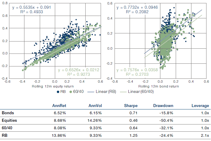
In Figure 3 we illustrate the results in an analogous fashion to Figure 2. Note how this risk-balanced approach:
- Correlates to equities less than 60/40 (48% versus 93%);
- Mitigates the downside in equity returns better than 60/40;
- Generates higher returns on average than 60/40 (14% versus 8%);
- Has a lower drawdown than 60/40 (24% versus 32%).
Note that the additional diversification afforded by an increased bond allocation in RB over 60/40 means that we have taken on leverage, in this case around 2.1x, in order to get to the same level of return volatility as 60/40. In doing so, however, returns have increased and drawdown has reduced. Leverage, in this case, should not be confused with risk.
Figure 3 illustrates the attractiveness of the risk-balanced approach over 60/40 from a historical perspective, but the key question facing investors is what is likely to happen in the future.
Figure 3. Rolling 12-Month Risk-Balanced (Blue) Versus 60/40 (Green) Returns as a Function of Equity Return (LHS) and Bond Return (RHS)
Simulated past performance is not indicative of future results. Returns may increase or decrease as a result of currency fluctuations.
Source: Man Group database, Bloomberg, MSCI. Date range: 1 January 1960 to 31 August 2020.
Simulated performance data and hypothetical results are shown for illustrative purposes only, do not reflect actual trading results, have inherent limitations and should not be relied upon. Results are gross of any fees or expenses which could materially reduce returns. Please see the end of this paper for additional important information on simulated results.
60/40 and Risk-Balanced Portfolios in 2020 and Beyond
60/40 has come in for a bit of stick in 2020. In March, marking the Covid-19 related nadir, a 60/40 investment in global equities and bonds was down 8.2%. Equities alone lost 12.6% and bonds lost 1.6%. In comparison, a simple risk-balanced approach lost 6.6%. This has not gone un-noticed by market participants and the media where the future of 60/40 has been brought into question.2
There are generally two themes presented for the bleak outlook. The first is that bonds and stocks are expensive, so now may not be a great time to invest in long-only products. The second theme is that, with bond yields at very low levels, there is doubt that bonds can still protect equity portfolios in a sell-off in ways they have done historically.
These two themes are not unrelated, in our view. The link lies in the observation that a cash bond’s total nominal return to maturity is capped at zero when yields go to zero, and yields in developed markets are either there already (Germany) or getting close to there (US). Conversely, while equities are expensive in price terms on a historic basis, they can theoretically get more expensive through, for example, multiple expansion. Hence, the real crux of the problem is bonds.
Given the perceived bleak outlook for bonds in an increasingly zero yield world, it might be tempting to revert to 60/40 rather than a risk-balanced approach, in light of 60/40’s lower bond allocation. As we illustrated in Figure 2, however, in reality, this means only a token bond allocation. Nevertheless, we believe that bonds can still play an important role in bond-equity portfolios for the following reasons.
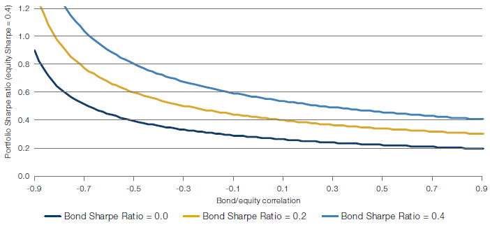
Although at first sight the risk-balanced approach is predicated on both long-term positive return assumptions and low or negative correlation of the instruments traded, the reality is a more nuanced combination of the two. To illustrate this, we conducted a synthetic study of two instruments with equal risk in a portfolio; let’s call them ‘bonds’ and ‘equities’. Figure 4 shows the effect of adding bonds, with varying Sharpe ratios3, to equities assuming equities have a Sharpe ratio of 0.4. The downward-sloping lines tell us that the value of bonds in multi-asset portfolios declines as correlation between bonds and equities increases. This is expected. More interestingly, perhaps, the chart shows that bonds can be additive to the portfolio at correlation <-0.5 even if their expected Sharpe ratio is zero.
Figure 4. Linking Bond/Equity Correlation and Sharpe Ratios Through a Synthetic Portfolio
Source: Man Group. Illustrative example – for information only.
Equities are assumed to have a Sharpe ratio of 0.4, and bonds and equities are equally risk weighted.
Another way to think of this is that in times of market stress, when we assume bonds and equities are most negatively correlated, bonds protect the portfolio and afford more exposure to both asset classes in the good times. In order to maximise this effect, we believe it makes sense to concentrate on the highest-quality fixed income instruments to maximise the flight-to-safety effect. As Figure 5 illustrates, over the Covid-19 episode in the first quarter of 2020, US Treasuries and German Bunds displayed yield declines at least initially while those of Italy did not.
Outside the scope of this article, but worth mentioning, is that there are other ways that a risk-balanced portfolio can be responsive to a changing environment for bonds. First, advanced correlation models (Shephard & Sheppard, 2012) can be used in order to de-risk portfolios when bonds and equities become positively correlated and multi-asset portfolios become more vulnerable to losses. This has become an increasing problem in the quantitative easing era, such as the Taper Tantrum episode in 2013 when US Treasury yields surged on the suggestion of the withdrawal of central bank support. Second, the use of bond futures can potentially mitigate the guaranteed flat return of a held-to-maturity zero yielding bond since a futures price is sensitive to the slope of the interest-rate curve around a given maturity point as opposed to the total yield to maturity.
Figure 5. Government Bond 10y Yield (Top) and Corresponding Equity Index Price (Bottom) Showing Initial Flight-To-Safety effect of Government Bonds in US, UK and Germany
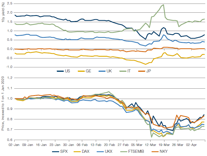
Source: Man Group database and Bloomberg. Date range: 2 January to 10 April 2020.
World equities represented by MSCI World Net Total Return Index (hedged to USD), world bonds by Barclays Capital Global Aggregate Bond Index (hedged to USD).
So risk-balanced portfolios with equities and bonds still have a role to play in the future, we believe, especially if they concentrate on high quality government bond futures and have active risk management. But there is more that can be done …
Improving Bond-Equity Portfolios
We realise that investors have options outside equities and bonds in a long-only framework in order to diversify returns. Investments in private equity and infrastructure are obvious candidates here, although portfolio liquidity will likely be compromised via this route. In addition, as Harvey et. al. (2017) point out, a tilt towards quality stocks can perform well in times of market stress. Sticking to the theme of this note, however, in this section, we concentrate on how the 60/40 portfolio could be adapted for a world where bonds and equities are expensive and bond price appreciation, in particular, is capped.
We have not stated it explicitly thus far, but the progression from 60/40 to risk-balanced involves a degree of active management. 60/40 investors only have to rebalance periodically in order to maintain those notional allocations when equities significantly outperform bonds, or vice versa. On top of this, a risk-balanced portfolio also has to adjust its positions to maintain the overall volatility of the portfolio, shrinking allocations when volatility is high, and scaling up when it is low. It also does all this on a levered basis; an average of 2.1, as we have found.
But we digress. The point here is that an investor can introduce active, risk-based market timing into the risk-balanced portfolio through volatility scaling. A second element of market timing that can be added is a correlation model, as we discussed in the previous section. This seeks to limit portfolio positions when bonds and equities are not diversifying each other as much as we would like. Another element that we believe can be of great help to bond-equity portfolios in the future is time-series momentum, or trend-following.
The seeds of the trend-following industry were sown in the late 1970s, so the strategy has established credentials and track record. Trend-following attempts to profit from trends, either up or down, in liquid markets across asset classes. By design, therefore, it should be lowly correlated to any one asset class, and should be able to profit from large moves as long as they occur in a sustained manner. Hamill et. al. (2017) investigated the performance of a simple trend-following strategy momCTA using data from 1960 which, unlike the live returns from the industry itself, incorporate the period in the 1970s and 1980s when interest rates rose.4 In Figure 6, we represent trend-following’s 12-month returns, using momCTA from January 1960 until we have industry data via the Barclay BTOP50 index in January 1987 to August 2020.
Figure 6. Rolling 1-Month Trend-Following (Grey) Versus 60/40 (Green) Returns as a Function of Equity Return (LHS) and Bond Return (RHS)
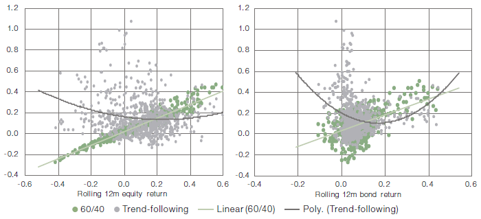
Source: Man Group database, Bloomberg, MSCI, BarclayHedge. Date range: 1 January 1960 to 31 August 2020.
There is clearly considerable scatter in the trend-following returns. This is expected given they are a function of prices in multiple asset classes, not just equities and bonds. The best-fit quadratic function does indeed hint at stronger returns at the extremes of market moves, and lowest nearer the centre of the charts where large market moves are absent. We have gone back to 1960 for our dataset in order to include a period of rising rates. However, the performance of the trend-following strategy during weak bond markets is poorly constrained, although it appears to be significantly superior to that of 60/40.
Readers can probably see where we are going with this. As Figure 6 shows, adding an allocation of trend-following to a long-only investment has the potential to mitigate the downside of portfolios consisting of long only investments in equities and bonds. Payback, if you like, is the relative underperformance of trend-following in the best of years; to the far right-hand side of both charts in the figure.
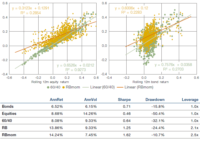
A small allocation to trend-following could be viewed as a tilt on the long-only portfolio, in that it is unlikely to take the aggregate position in bonds or equities short. In Figure 7, we illustrate the effect of a 25% notional allocation to trend following coupled with a 75% allocation to the risk-balanced strategy, which we term 'RBmom’. In our experience, this is enough to occasionally take the aggregate bond position short in times of extreme bond market stress such as 2013’s Taper Tantrum, discussed earlier.
The table in Figure 7 illustrates that adding trend-following improves the return, decreases volatility, and reduces drawdown relative to the risk-balanced portfolio alone, and both actively managed portfolios are significant improvements over 60/40.
Figure 7. Rolling 12-Month Return of RBmom (Orange) Versus 60/40 (Green) Returns as a Function of Equity Return (LHS) and Bond Return (RHS)
Simulated past performance is not indicative of future results. Returns may increase or decrease as a result of currency fluctuations.
Source: Man Group database, Bloomberg, MSCI. Date range: 1 January 1960 to 31 August 2020.
Monthly return of RBmom (orange), consisting of 75% risk balanced and 25% trend following, versus 60/40 (green) returns.
Simulated performance data and hypothetical results are shown for illustrative purposes only, do not reflect actual trading results, have inherent limitations and should not be relied upon. Results are gross of any fees or expenses which could materially reduce returns. Please see the end of this paper for additional important information on simulated results.
Summary and Conclusion
60/40 has served investors well, particularly in light of the performance of both stocks and bonds over recent decades. As the table in Figure 7 shows, 60/40 gave equity-like returns for around two-thirds of the risk of an equity investment alone and a substantially reduced drawdown. With a less rosy outlook for equities and bonds, however, we believe investors have to go active. To start with, a risk-balanced approach introduces a first layer of active management, namely responsiveness to market volatility. Trend-following adds a market timing element, further reducing risk when a given market’s price declines.
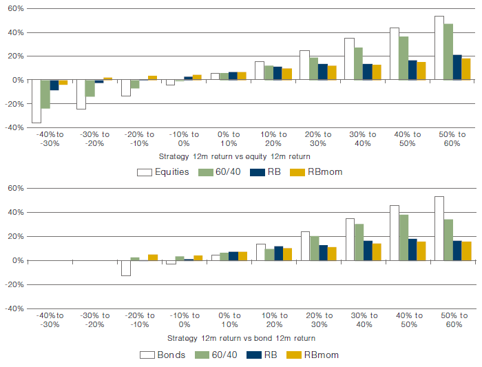
Figure 8 summarises the various iterations to improve 60/40 that we have proposed in this article, and presents them in a way that may help investors when they consider future scenarios. We stick to the same colour schemes; green for 60/40, blue for risk-balanced, and orange for risk-balanced + momentum (RBmom). In order to facilitate direct comparisons we have scaled the returns across the sample period for all variants to be the same, at 8%, which is what our equity dataset annualises.
In the top chart, we consider the distribution of 12-month rolling returns as a function of equity market rolling 12-month return. The white bars just act to show what a straight equities investment would look like. As we saw in Figure 2, 60/40 behaves just like equities, because that is where the risk in 60/40 lies. Risk-balanced, in blue, does significantly better than 60/40 on the downside, but less well on the upside. Adding 25% trend-following, in orange, means losses are experienced only when equities lose 30-40% over a 12-month basis, although the upside at higher equity returns is slightly reduced.
Figure 8. Distribution of Rolling 12-Month Returns for Various Portfolios Discussed in This Article
Simulated past performance is not indicative of future results. Returns may increase or decrease as a result of currency fluctuations.
Source: Man Group database, Bloomberg, MSCI. Date range: 1 January 1960 to 31 August 2020.
All are normalised to return 8% per annum. Presented as a function of 12-month equity return (top) and 12-month bond return, bottom. Simulated performance data and hypothetical results are shown for illustrative purposes only, do not reflect actual trading results, have inherent limitations and should not be relied upon. Results are gross of any fees or expenses which could materially reduce returns. Please see the end of this paper for additional important information on simulated results.
A similar effect is seen viewed through the lens of bonds in the lower half of Figure 8. RBmom becomes a better proposition the worse bond 12-month performance gets. Although we do not have the same coverage, in terms of bond market drawdown, as we do for equities, the fact that patterns in both cases are consistent gives us some confidence that RBmom might behave in a similar way for extreme bond market down-moves as it does for extreme equity market down-moves.
Figure 8 can act as a roadmap for investors to implement their view of the future. If we assume that, in the future, bond and equity price moves are drawn from the same distribution as Figure 8, an investor can choose a portfolio based on their view of the world. With a rosy view for equities and bonds, the investor might concentrate on the right-hand-side of the distributions and probably stick to 60/40. We would point out, however, that this comment probably only holds when we expect equities (or scaled bonds) to make in excess of 20% per annum. For more moderate scenarios, or for investors with a bearish view, however, the data suggests a focus toward the left and a move towards RBmom.
RBmom has a somewhat arbitrary 25% momentum allocation. How much trend-following to add depends on how pessimistic the view of the future is, or how tolerant an investor is of drawdowns. The analysis which we have presented here suggests that long-term investors who are concerned about expensive bonds and equities should consider some trend-following in their portfolios. Similarly, investors with only a short time to retirement and therefore greater sensitivity to drawdowns, may also find trend-following a valuable addition to their long-only exposure.
To summarise, it would seem that the longevity of 60/40 is predicated by continued performance of equities in particular. For other scenarios, we believe investors have options if they embrace active management via risk rather than notional investing, and market-timing overlays such as trend-following.
1. We scale bond and equity returns by the ratio of target volatility to realised volatility over the previous 12 months and cap leverage at 4x.
2. “Investors wonder if the 60/40 portfolio has a future”, Financial Times, 22 September 2020.
3. Sharpe ratio is a measure of risk-adjusted performance that indicates the level of excess return per unit of risk. It is calculated using the risk-free rate (3 month interbank rate) in the appropriate currency over the period analysed.
4. Where momCTA overlaps with the Barclay BTOP50 index of trend-followers the correlation of monthly returns is 0.63.
Bibliography
Harvey, C. R., E. Hoyle, S. Rattray, M. Sargaison, D. Taylor, and O. Van Hemert (2019), “The Best of Strategies for the Worst of Times: Can Portfolios Be Crisis Proofed”. The Journal of Portfolio Management, July 2019, 45 (5) 7-28; DOI: https://doi.org/10.3905/jpm.2019.45.5.007
Rattray, S., N. Granger, C. R. Harvey, and O. Van Hemert (2020), “Strategic Rebalancing”, The Journal of Portfolio Management Multi-Asset Special Issue 2020, jpm.2020.1.150; DOI: https://doi.org/10.3905/jpm.2020.1.150.
Hamill, C., S. Rattray, and O. Van Hemert, “Trend Following: Equity and Bond Crisis Alpha” (August 30, 2016). Available at SSRN: https://ssrn.com/abstract=2831926
Harvey, C. R., E. Hoyle, R. Korgaonkar, S. Rattray, M. Sargaison, and O. Van Hemert (2018), “The impact of volatility targeting”, Journal of Portfolio Management, 45(1), 14-33.
Noureldin, D., N. Shephard, K. Sheppard (2012), “Multivariate high-frequency-based volatility (HEAVY) models”, Journal of Applied Econometrics, 27(6), 907-933.
Shephard, N., K. Sheppard (2010), “Realising the future: forecasting with high-frequency-based (HEAVY) models”, Journal of Applied Econometrics, 25(2), 197-231.
Hypothetical Results
Hypothetical Results are calculated in hindsight, invariably show positive rates of return, and are subject to various modelling assumptions, statistical variances and interpretational differences. No representation is made as to the reasonableness or accuracy of the calculations or assumptions made or that all assumptions used in achieving the results have been utilized equally or appropriately, or that other assumptions should not have been used or would have been more accurate or representative. Changes in the assumptions would have a material impact on the Hypothetical Results and other statistical information based on the Hypothetical Results.
The Hypothetical Results have other inherent limitations, some of which are described below. They do not involve financial risk or reflect actual trading by an Investment Product, and therefore do not reflect the impact that economic and market factors, including concentration, lack of liquidity or market disruptions, regulatory (including tax) and other conditions then in existence may have on investment decisions for an Investment Product. In addition, the ability to withstand losses or to adhere to a particular trading program in spite of trading losses are material points which can also adversely affect actual trading results. Since trades have not actually been executed, Hypothetical Results may have under or over compensated for the impact, if any, of certain market factors. There are frequently sharp differences between the Hypothetical Results and the actual results of an Investment Product. No assurance can be given that market, economic or other factors may not cause the Investment Manager to make modifications to the strategies over time. There also may be a material difference between the amount of an Investment Product’s assets at any time and the amount of the assets assumed in the Hypothetical Results, which difference may have an impact on the management of an Investment Product. Hypothetical Results should not be relied on, and the results presented in no way reflect skill of the investment manager. A decision to invest in an Investment Product should not be based on the Hypothetical Results.
No representation is made that an Investment Product’s performance would have been the same as the Hypothetical Results had an Investment Product been in existence during such time or that such investment strategy will be maintained substantially the same in the future; the Investment Manager may choose to implement changes to the strategies, make different investments or have an Investment Product invest in other investments not reflected in the Hypothetical Results or vice versa. To the extent there are any material differences between the Investment Manager’s management of an Investment Product and the investment strategy as reflected in the Hypothetical Results, the Hypothetical Results will no longer be as representative, and their illustration value will decrease substantially. No representation is made that an Investment Product will or is likely to achieve its objectives or results comparable to those shown, including the Hypothetical Results, or will make any profit or will be able to avoid incurring substantial losses. Past performance is not indicative of future results and simulated results in no way reflect upon the manager’s skill or ability.
You are now leaving Man Group’s website
You are leaving Man Group’s website and entering a third-party website that is not controlled, maintained, or monitored by Man Group. Man Group is not responsible for the content or availability of the third-party website. By leaving Man Group’s website, you will be subject to the third-party website’s terms, policies and/or notices, including those related to privacy and security, as applicable.