Covering Your Tail: The Case for Expected Shortfall in Tail Risk Management

Key takeaways:

• Variance is the most commonly used measure of portfolio risk, but there are compelling alternatives
• Expected shortfall, sometimes called conditional value-at-risk (CVaR), retains many of variance’s most useful properties, while surmounting key shortcomings
• We demonstrate how CVaR can be employed to combine return streams with complementary left-tail properties when building market-neutral equity strategies. Doing so aims to moderate portfolio drawdowns and help insulate investors from model-specific adverse events

Introduction

Variance remains the most widely used measure of portfolio risk across the investment industry, yet its dominance belies important limitations. At Man Numeric, we believe there exist alternative measures which may offer a more compelling way to manage extreme tail risk. One of those is expected shortfall, sometimes called conditional value-at-risk (CVaR), which retains many of variance’s most useful properties, while surmounting key shortcomings. This paper explores some of the ways expected shortfall improves on variance for risk management and explains how it can be leveraged for model allocation in systematic equities portfolios.

The trouble with variance

In 1952, Harry Markowitz invented Modern Portfolio Theory (MPT) by formalising a bedrock principle in finance: when faced with portfolios of equal expected returns, risk-averse investors will naturally prefer the one with the lowest risk. He expressed this idea mathematically as the mean-variance optimisation, which trades off expected return and volatility (i.e., the square root of variance). This began variance’s more than 70-year reign as the de rigueur measure of portfolio risk.

Yet despite its many merits, variance is flawed. It does a fairly poor job of proxying extreme downside risk, because it treats all returns as risky. A portfolio that only ever gains value may be, from the standpoint of variance, just as risky as one that only ever loses it. This is a provocative framing, but it reveals something important about what variance misses.

Consider Figure 1 below, which plots two synthetic price series of equal expected return and variance. From the standpoint of mean-variance optimisation they are, by construction, equally attractive. It is clear, however, that these portfolios are not equal. Portfolio Two is much “crashier”; its long-run trend is equivalent to that of Portfolio One, but its history is full of unpredictable booms and busts. By contrast, Portfolio One offers a smoother ride. Although it is locally volatile, it lacks Portfolio Two’s severe downward swings.

Figure 1: Equal variance but unequal risk

Problems loading this infographic? - Please click here

Source: Man Numeric, as at July 2025.

We can visualise these differences by plotting how far each portfolio has fallen from its high water mark at each moment in time. This measure, called “drawdown”, reveals Portfolio Two’s propensity for adverse events. Several times in its history Portfolio Two suddenly loses more than 10% of its total value. In Portfolio One, that happens just once.

Figure 2: Distinct drawdown properties

Problems loading this infographic? - Please click here

Source: Man Numeric, as at July 2025.

Investors who prefer Portfolio One’s return stream are not well served by variance, which is unable to discriminate between Portfolios One and Two. Unfortunately, the difference in downside risk which distinguishes them is invisible to variance. We need another measure.

Enter expected shortfall

Expected shortfall, or CVaR, aims to measure the loss associated with just the very worst returns. A cousin of the perhaps more familiar value-at-risk (VaR), expected shortfall is formally defined as follows: where α is the value-at-risk threshold, N is the sample size, and r_(i) is the i^th ordered return.

In the simplest terms, the formula proposes ordering daily returns from worst to best and averaging the bottom α percent of them. For an asset with the return distribution shown below in Figure 3, if we set α equal to 40%, CVaR_0.4 is the average of the worst 40% of daily returns. This is the light blue area to the left of α.

Figure 3: Visualising expected shortfall

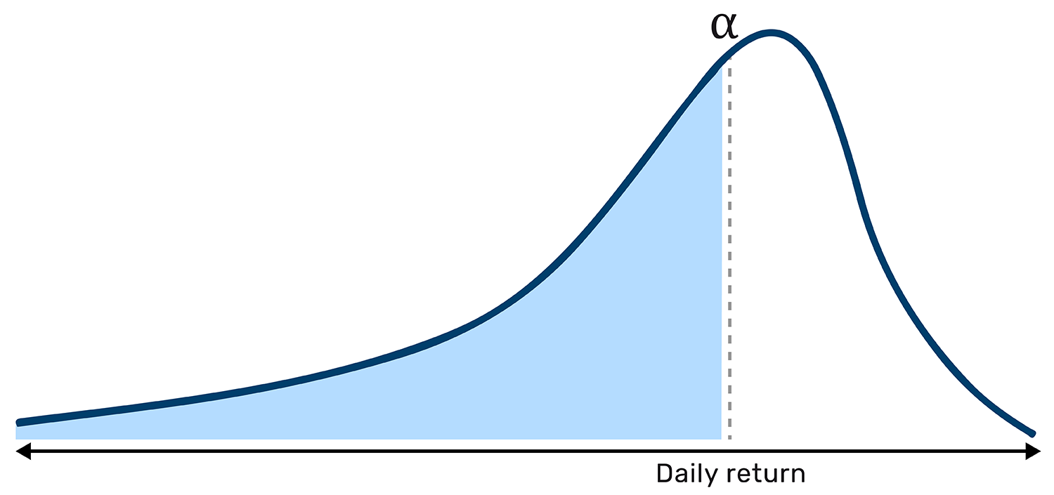
Schematic illustration. Source: Man Numeric.

Already, this simple diagram illuminates one of the advantages of expected shortfall – it explicitly measures adverse outcomes. Applied to the return streams above, it readily differentiates between Portfolio One (with a CVaR_0.4 of -1.32%) and Portfolio Two (with a CVaR_0.4 of -1.78%). These figures tell us that the performance of Portfolio One on its worst 40% of days is more than 25% better than Portfolio Two on its worst days. Notwithstanding the portfolios’ equal variance and expected return, when Portfolio Two has a bad day, it has a really bad day!

While the drawdown plots in Figure 2 already hint at Portfolio One’s superior left-tail properties, the advantage of expected shortfall is that it maintains many of variance’s most useful properties. It is convex, computationally tractable, and reasonably persistent given practical sample sizes. Because of these features, expected shortfall can be used in place of, or as a supplement to, variance in many optimisation tasks.

Expected shortfall in allocation

Imagine that on 14 December 2016 – or any other date we might choose – we want to produce a portfolio which, over the next six months, has the best possible risk-return trade off. We randomly select 20 large-cap, global stocks and assign long-only weights which sum to one. To determine our weights we could construct the minimum variance portfolio using the returns from the last five years. Alternatively, we could use CVaR_0.4 as our risk measure and thereby construct the minimum shortfall portfolio. Running these portfolios forward (out-of-sample) produces the results shown in Figure 4.

Figure 4: Comparative out-of-sample performance

Problems loading this infographic? - Please click here

Source: Man Numeric, as at 8 June 2017.

Clearly the shortfall-minimising portfolio produces a better average return during the out-of-sample period. This may be partly because unlike variance, expected shortfall does not penalise outperformance on the upside. The shortfall-minimising portfolio also has slightly lower out-of-sample volatility (7.2% annualised versus 7.4%). But since investors might care more about downside risk than daily volatility, a metric like the drawdown ratio has intuitive appeal. According to this measure, which is simply annual return divided by unsigned maximum drawdown, the shortfall-minimising portfolio once again outperforms the minimum-variance portfolio, though only slightly: 14.9 to 13.9.

While suggestive, these results are not dispositive. Expected shortfall might outperform variance for this period and set of securities but underperform generally. We might have more conviction in the use of expected shortfall if we repeated the experiment a few more times across different periods and groups of stocks.

Figure 5: Comparing drawdown ratios over ~25 years

Problems loading this infographic? - Please click here

Source: Man Numeric, as at July 2025.

Figure 5 plots the results of more than one million trials. Each consists of randomly selecting 20 large-cap, global stocks and choosing an optimisation date between 31 October 2000 and 29 August 2024 without bias. Although the difference in drawdown ratio is modest – 26.7 for minimum shortfall versus 26.0 for minimum variance – its replicability points to a tendency for shortfall-minimising portfolios to deliver better returns per unit of drawdown than their variance-minimising counterparts. And perhaps most importantly, small differences delivered consistently, really add up!

Leveraging expected shortfall in systematic equity portfolios

For investors concerned with the trade-off between expected gain and extreme loss, these results suggest shortfall-aware portfolio optimisation techniques might drive real benefit to their portfolios. There is, however, a practical challenge. When estimating the statistical properties of a distribution, more data are better than fewer. Regrettably, expected shortfall is data intensive. Although we might prefer CVaR_0.05 or even CVaR_0.01, we typically lack sufficient return history to make these measures practical. Even CVaR_0.4, which relies on 40% of available returns, may, depending on context, require more history than is realistic.

For this reason, expected shortfall is often best utilised for tasks where the number of quantities estimated is small or the history is long. That may rule out many direct portfolio construction applications, especially in equities, but it remains valuable in signal allocation.

Like portfolio construction, signal allocation seeks to identify target weights which impart beneficial properties to portfolios. In the case of signal allocation, those weights are applied to alpha signal returns rather than individual securities. So while an investable universe might contain thousands of stocks, a portfolio typically contains just dozens of models. Provided there is a reasonable history, robust optimisation is usually feasible.

Just how much benefit might a portfolio derive from allocating via expected shortfall? Under the right circumstances, quite a lot. Figure 6 below plots the drawdowns of three signals which we might wish to combine. Given that we are chiefly concerned about extreme loss, we choose allocations via an expected shortfall optimisation. The resulting return stream radically outperforms its constituents. Adjusting for volatility, the maximum peak-to-trough drawdowns are -15.9% for Signal One, -12.8% for Signal Two, and -25.6% for Signal Three. For the expected shortfall-optimised return stream, on the other hand, the figure is -9.8%. If we had minimised variance instead, we would have realised a maximum drawdown of -15.6%. Equal weighting would have yielded -18.9%.

Figure 6: Reducing drawdown via allocation

Problems loading this infographic? - Please click here

Source: Man Numeric, as at July 2025.

An important reason expected shortfall performs the way it does in this example is, that for these signals, expected shortfall is a reasonably good proxy for drawdown. By minimising the expected shortfall of the resulting portfolio, we are indirectly combining the drawdown profiles of our constituent signals so that in any given period drawdowns in one are offset by profitability in the others. With just three signals, we might have some inkling about which allocation might work best for this purpose. With tens or hundreds of signals, the task is harder. This is one of the chief benefits of using expected shortfall for allocation.

Yet despite its advantages, expected shortfall is not a panacea for all sources of left-tail risk. Like most statistical measures, it requires substantial data and can be sensitive to parameterisation (e.g., how much history and what percentage of returns are used to compute it). What’s more, not all distributions are equally distinguishable via expected shortfall. Its value is most obvious in cases where the originating distribution is asymmetric with long, fat tails (like the signals in Figure 6) or non-linear payoffs. Indeed, when returns are believed to be symmetric, variance often remains a better choice, since it’s estimated over the full sample. Perhaps worst of all, optimising with expected shortfall does little to protect against long, slow drawdowns characterised by serially correlated returns.

To capture its benefits while sidestepping its limitations, Man Numeric employs expected shortfall in combination with other risk estimation techniques as part of an ensemble. Our allocation framework attempts to match our investors’ utility functions by balancing expected return against various risk dimensions, of which extreme downside is probably the most important. Combining models with complementary left-tail properties can help to moderate portfolio drawdowns and insulate investors from model-specific adverse events. Expected shortfall is valuable, because it proxies downside risk, and, unlike many other left-tail targeting risk measures like value-at-risk or maximum drawdown, its convexity ensures speedy optimisation.

Conclusion: Combining risk measures for improved outcomes

While variance has long served as the dominant measure of portfolio risk, CVaR better targets extreme loss in many cases. In so doing, it better aligns with many investors' aversion to left-tail risk. And although the metric is not perfect, it is compatible with other risk measures, so it lends itself to ensemble-based approaches. That is why, in building market neutral content at Man Numeric, we employ it beside, and in combination with, other risk estimation techniques. This approach better reflects the diverse sources of risk investors care about and makes explicit the return trade-off required to mitigate these risks in an equity portfolio.